
| | |  Посмотреть исходный код на GitHub Посмотреть исходный код на GitHub | |
Обзор
Premade Модель быстро и легко способы построения TFL tf.keras.model экземпляров для типичных случаев использования. В этом руководстве описаны шаги, необходимые для создания готовой модели TFL и ее обучения/тестирования.
Настраивать
Установка пакета TF Lattice:
pip install tensorflow-lattice pydot
Импорт необходимых пакетов:
import tensorflow as tf

import copy
import logging
import numpy as np
import pandas as pd
import sys
import tensorflow_lattice as tfl
logging.disable(sys.maxsize)
Установка значений по умолчанию, используемых для обучения в этом руководстве:
LEARNING_RATE = 0.01
BATCH_SIZE = 128
NUM_EPOCHS = 500
PREFITTING_NUM_EPOCHS = 10
Загрузка набора данных UCI Statlog (Heart):
heart_csv_file = tf.keras.utils.get_file(
    'heart.csv',
    'http://storage.googleapis.com/download.tensorflow.org/data/heart.csv')
heart_df = pd.read_csv(heart_csv_file)
thal_vocab_list = ['normal', 'fixed', 'reversible']
heart_df['thal'] = heart_df['thal'].map(
    {v: i for i, v in enumerate(thal_vocab_list)})
heart_df = heart_df.astype(float)

heart_train_size = int(len(heart_df) * 0.8)
heart_train_dict = dict(heart_df[:heart_train_size])
heart_test_dict = dict(heart_df[heart_train_size:])

# This ordering of input features should match the feature configs. If no
# feature config relies explicitly on the data (i.e. all are 'quantiles'),
# then you can construct the feature_names list by simply iterating over each
# feature config and extracting it's name.
feature_names = [
    'age', 'sex', 'cp', 'chol', 'fbs', 'trestbps', 'thalach', 'restecg',
    'exang', 'oldpeak', 'slope', 'ca', 'thal'
]

# Since we have some features that manually construct their input keypoints,
# we need an index mapping of the feature names.
feature_name_indices = {name: index for index, name in enumerate(feature_names)}

label_name = 'target'
heart_train_xs = [
    heart_train_dict[feature_name] for feature_name in feature_names
]
heart_test_xs = [heart_test_dict[feature_name] for feature_name in feature_names]
heart_train_ys = heart_train_dict[label_name]
heart_test_ys = heart_test_dict[label_name]
Downloading data from http://storage.googleapis.com/download.tensorflow.org/data/heart.csv
16384/13273 [=====================================] - 0s 0us/step
24576/13273 [=======================================================] - 0s 0us/step
Конфигурации функций
Калибровка Характеристики и в-функции конфигурация устанавливаются с помощью tfl.configs.FeatureConfig . Конфигурации включают Feature монотонности ограничения, в-функцию упорядочению (см tfl.configs.RegularizerConfig ) и решетку размеры для решетчатых моделей.
Обратите внимание, что мы должны полностью указать конфигурацию функции для любой функции, которую мы хотим, чтобы наша модель распознала. В противном случае модель не сможет узнать о существовании такой функции.
Определение наших конфигураций функций
Теперь, когда мы можем вычислить наши квантили, мы определяем конфигурацию функции для каждой функции, которую мы хотим, чтобы наша модель принимала в качестве входных данных.
# Features:
# - age
# - sex
# - cp        chest pain type (4 values)
# - trestbps  resting blood pressure
# - chol      serum cholestoral in mg/dl
# - fbs       fasting blood sugar > 120 mg/dl
# - restecg   resting electrocardiographic results (values 0,1,2)
# - thalach   maximum heart rate achieved
# - exang     exercise induced angina
# - oldpeak   ST depression induced by exercise relative to rest
# - slope     the slope of the peak exercise ST segment
# - ca        number of major vessels (0-3) colored by flourosopy
# - thal      normal; fixed defect; reversable defect
#
# Feature configs are used to specify how each feature is calibrated and used.
heart_feature_configs = [
    tfl.configs.FeatureConfig(
        name='age',
        lattice_size=3,
        monotonicity='increasing',
        # We must set the keypoints manually.
        pwl_calibration_num_keypoints=5,
        pwl_calibration_input_keypoints='quantiles',
        pwl_calibration_clip_max=100,
        # Per feature regularization.
        regularizer_configs=[
            tfl.configs.RegularizerConfig(name='calib_wrinkle', l2=0.1),
        ],
    ),
    tfl.configs.FeatureConfig(
        name='sex',
        num_buckets=2,
    ),
    tfl.configs.FeatureConfig(
        name='cp',
        monotonicity='increasing',
        # Keypoints that are uniformly spaced.
        pwl_calibration_num_keypoints=4,
        pwl_calibration_input_keypoints=np.linspace(
            np.min(heart_train_xs[feature_name_indices['cp']]),
            np.max(heart_train_xs[feature_name_indices['cp']]),
            num=4),
    ),
    tfl.configs.FeatureConfig(
        name='chol',
        monotonicity='increasing',
        # Explicit input keypoints initialization.
        pwl_calibration_input_keypoints=[126.0, 210.0, 247.0, 286.0, 564.0],
        # Calibration can be forced to span the full output range by clamping.
        pwl_calibration_clamp_min=True,
        pwl_calibration_clamp_max=True,
        # Per feature regularization.
        regularizer_configs=[
            tfl.configs.RegularizerConfig(name='calib_hessian', l2=1e-4),
        ],
    ),
    tfl.configs.FeatureConfig(
        name='fbs',
        # Partial monotonicity: output(0) <= output(1)
        monotonicity=[(0, 1)],
        num_buckets=2,
    ),
    tfl.configs.FeatureConfig(
        name='trestbps',
        monotonicity='decreasing',
        pwl_calibration_num_keypoints=5,
        pwl_calibration_input_keypoints='quantiles',
    ),
    tfl.configs.FeatureConfig(
        name='thalach',
        monotonicity='decreasing',
        pwl_calibration_num_keypoints=5,
        pwl_calibration_input_keypoints='quantiles',
    ),
    tfl.configs.FeatureConfig(
        name='restecg',
        # Partial monotonicity: output(0) <= output(1), output(0) <= output(2)
        monotonicity=[(0, 1), (0, 2)],
        num_buckets=3,
    ),
    tfl.configs.FeatureConfig(
        name='exang',
        # Partial monotonicity: output(0) <= output(1)
        monotonicity=[(0, 1)],
        num_buckets=2,
    ),
    tfl.configs.FeatureConfig(
        name='oldpeak',
        monotonicity='increasing',
        pwl_calibration_num_keypoints=5,
        pwl_calibration_input_keypoints='quantiles',
    ),
    tfl.configs.FeatureConfig(
        name='slope',
        # Partial monotonicity: output(0) <= output(1), output(1) <= output(2)
        monotonicity=[(0, 1), (1, 2)],
        num_buckets=3,
    ),
    tfl.configs.FeatureConfig(
        name='ca',
        monotonicity='increasing',
        pwl_calibration_num_keypoints=4,
        pwl_calibration_input_keypoints='quantiles',
    ),
    tfl.configs.FeatureConfig(
        name='thal',
        # Partial monotonicity:
        # output(normal) <= output(fixed)
        # output(normal) <= output(reversible)
        monotonicity=[('normal', 'fixed'), ('normal', 'reversible')],
        num_buckets=3,
        # We must specify the vocabulary list in order to later set the
        # monotonicities since we used names and not indices.
        vocabulary_list=thal_vocab_list,
    ),
]
Установите монотонности и ключевые точки
Затем нам нужно правильно установить монотонность для функций, в которых мы использовали пользовательский словарь (например, «thal» выше).
tfl.premade_lib.set_categorical_monotonicities(heart_feature_configs)
Наконец, мы можем завершить настройку наших функций, вычислив и установив ключевые точки.
feature_keypoints = tfl.premade_lib.compute_feature_keypoints(
    feature_configs=heart_feature_configs, features=heart_train_dict)
tfl.premade_lib.set_feature_keypoints(
    feature_configs=heart_feature_configs,
    feature_keypoints=feature_keypoints,
    add_missing_feature_configs=False)
Калиброванная линейная модель
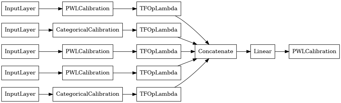
Для построения модели Premade TFL, сначала построить конфигурацию модели из tfl.configs . Калиброванная линейная модель построена с использованием tfl.configs.CalibratedLinearConfig . Он применяет кусочно-линейную и категориальную калибровку входных объектов, за которыми следует линейная комбинация и необязательная выходная кусочно-линейная калибровка. При использовании калибровки выходных данных или при задании выходных границ линейный слой будет применять взвешенное усреднение к откалиброванным входным данным.
В этом примере создается калиброванная линейная модель для первых 5 функций.
# Model config defines the model structure for the premade model.
linear_model_config = tfl.configs.CalibratedLinearConfig(
    feature_configs=heart_feature_configs[:5],
    use_bias=True,
    output_calibration=True,
    output_calibration_num_keypoints=10,
    # We initialize the output to [-2.0, 2.0] since we'll be using logits.
    output_initialization=np.linspace(-2.0, 2.0, num=10),
    regularizer_configs=[
        # Regularizer for the output calibrator.
        tfl.configs.RegularizerConfig(name='output_calib_hessian', l2=1e-4),
    ])
# A CalibratedLinear premade model constructed from the given model config.
linear_model = tfl.premade.CalibratedLinear(linear_model_config)
# Let's plot our model.
tf.keras.utils.plot_model(linear_model, show_layer_names=False, rankdir='LR')
2022-01-14 12:36:31.295751: E tensorflow/stream_executor/cuda/cuda_driver.cc:271] failed call to cuInit: CUDA_ERROR_NO_DEVICE: no CUDA-capable device is detected
Теперь, как и с любой другой tf.keras.Model , мы собираем и подобрать модель для наших данных.
linear_model.compile(
    loss=tf.keras.losses.BinaryCrossentropy(from_logits=True),
    metrics=[tf.keras.metrics.AUC(from_logits=True)],
    optimizer=tf.keras.optimizers.Adam(LEARNING_RATE))
linear_model.fit(
    heart_train_xs[:5],
    heart_train_ys,
    epochs=NUM_EPOCHS,
    batch_size=BATCH_SIZE,
    verbose=False)
<keras.callbacks.History at 0x7fe4385f0290>
После обучения нашей модели мы можем оценить ее на нашем тестовом наборе.
print('Test Set Evaluation...')
print(linear_model.evaluate(heart_test_xs[:5], heart_test_ys))
Test Set Evaluation...
2/2 [==============================] - 0s 3ms/step - loss: 0.4728 - auc: 0.8252
[0.47278329730033875, 0.8251879215240479]
Калиброванная модель решетки
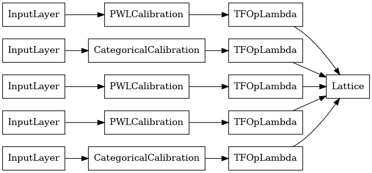
Калиброванные решетки модель построена с использованием tfl.configs.CalibratedLatticeConfig . Калиброванная решетчатая модель применяет кусочно-линейную и категориальную калибровку к входным объектам, за которыми следует решетчатая модель и необязательная выходная кусочно-линейная калибровка.
В этом примере создается калиброванная решетчатая модель для первых 5 объектов.
# This is a calibrated lattice model: inputs are calibrated, then combined
# non-linearly using a lattice layer.
lattice_model_config = tfl.configs.CalibratedLatticeConfig(
    feature_configs=heart_feature_configs[:5],
    # We initialize the output to [-2.0, 2.0] since we'll be using logits.
    output_initialization=[-2.0, 2.0],
    regularizer_configs=[
        # Torsion regularizer applied to the lattice to make it more linear.
        tfl.configs.RegularizerConfig(name='torsion', l2=1e-2),
        # Globally defined calibration regularizer is applied to all features.
        tfl.configs.RegularizerConfig(name='calib_hessian', l2=1e-2),
    ])
# A CalibratedLattice premade model constructed from the given model config.
lattice_model = tfl.premade.CalibratedLattice(lattice_model_config)
# Let's plot our model.
tf.keras.utils.plot_model(lattice_model, show_layer_names=False, rankdir='LR')
Как и раньше, мы компилируем, подгоняем и оцениваем нашу модель.
lattice_model.compile(
    loss=tf.keras.losses.BinaryCrossentropy(from_logits=True),
    metrics=[tf.keras.metrics.AUC(from_logits=True)],
    optimizer=tf.keras.optimizers.Adam(LEARNING_RATE))
lattice_model.fit(
    heart_train_xs[:5],
    heart_train_ys,
    epochs=NUM_EPOCHS,
    batch_size=BATCH_SIZE,
    verbose=False)
print('Test Set Evaluation...')
print(lattice_model.evaluate(heart_test_xs[:5], heart_test_ys))
Test Set Evaluation...
2/2 [==============================] - 1s 3ms/step - loss: 0.4709 - auc_1: 0.8302
[0.4709009826183319, 0.8302004933357239]
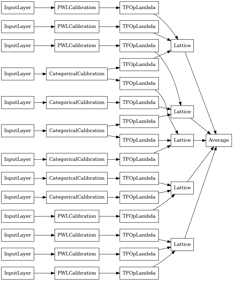
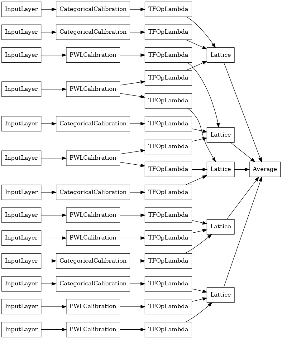
Калиброванная модель решетчатого ансамбля
Когда число функций велико, вы можете использовать ансамблевую модель, которая создает несколько меньших решеток для подмножеств функций и усредняет их выходные данные вместо создания одной огромной решетки. Ансамбль решетчатые модели построены с использованием tfl.configs.CalibratedLatticeEnsembleConfig . Модель ансамбля калиброванной решетки применяет кусочно-линейную и категориальную калибровку входного объекта, за которой следует ансамбль моделей решетки и необязательная выходная кусочно-линейная калибровка.
Явная инициализация ансамбля решеток
Если вы уже знаете, какие подмножества функций вы хотите передать в свои решетки, вы можете явно задать решетки, используя имена функций. В этом примере создается калиброванная модель ансамбля решеток с 5 решетками и 3 элементами на решетку.
# This is a calibrated lattice ensemble model: inputs are calibrated, then
# combined non-linearly and averaged using multiple lattice layers.
explicit_ensemble_model_config = tfl.configs.CalibratedLatticeEnsembleConfig(
    feature_configs=heart_feature_configs,
    lattices=[['trestbps', 'chol', 'ca'], ['fbs', 'restecg', 'thal'],
              ['fbs', 'cp', 'oldpeak'], ['exang', 'slope', 'thalach'],
              ['restecg', 'age', 'sex']],
    num_lattices=5,
    lattice_rank=3,
    # We initialize the output to [-2.0, 2.0] since we'll be using logits.
    output_initialization=[-2.0, 2.0])
# A CalibratedLatticeEnsemble premade model constructed from the given
# model config.
explicit_ensemble_model = tfl.premade.CalibratedLatticeEnsemble(
    explicit_ensemble_model_config)
# Let's plot our model.
tf.keras.utils.plot_model(
    explicit_ensemble_model, show_layer_names=False, rankdir='LR')
Как и раньше, мы компилируем, подгоняем и оцениваем нашу модель.
explicit_ensemble_model.compile(
    loss=tf.keras.losses.BinaryCrossentropy(from_logits=True),
    metrics=[tf.keras.metrics.AUC(from_logits=True)],
    optimizer=tf.keras.optimizers.Adam(LEARNING_RATE))
explicit_ensemble_model.fit(
    heart_train_xs,
    heart_train_ys,
    epochs=NUM_EPOCHS,
    batch_size=BATCH_SIZE,
    verbose=False)
print('Test Set Evaluation...')
print(explicit_ensemble_model.evaluate(heart_test_xs, heart_test_ys))
Test Set Evaluation...
2/2 [==============================] - 1s 4ms/step - loss: 0.3768 - auc_2: 0.8954
[0.3768467903137207, 0.895363450050354]
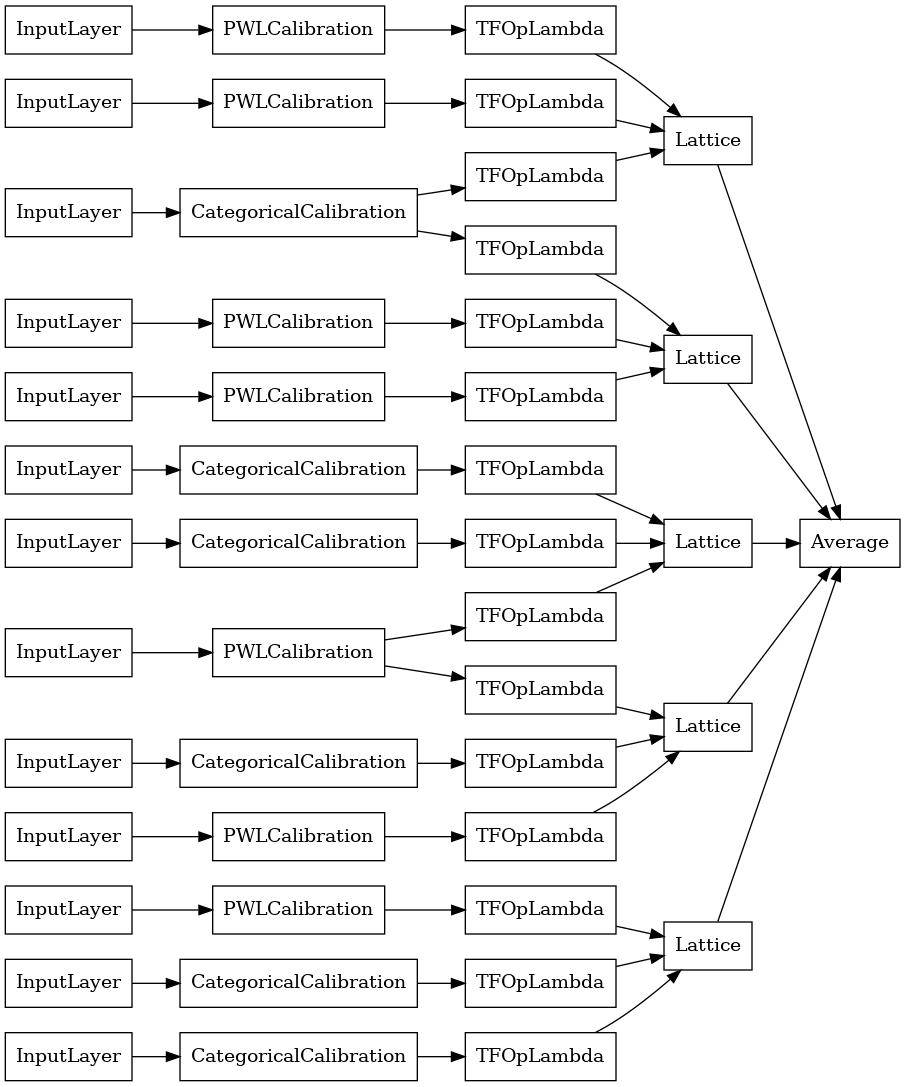
Случайный ансамбль решеток
Если вы не уверены, какие подмножества объектов вводить в свои решетки, другой вариант — использовать случайные подмножества признаков для каждой решетки. В этом примере создается калиброванная модель ансамбля решеток с 5 решетками и 3 элементами на решетку.
# This is a calibrated lattice ensemble model: inputs are calibrated, then
# combined non-linearly and averaged using multiple lattice layers.
random_ensemble_model_config = tfl.configs.CalibratedLatticeEnsembleConfig(
    feature_configs=heart_feature_configs,
    lattices='random',
    num_lattices=5,
    lattice_rank=3,
    # We initialize the output to [-2.0, 2.0] since we'll be using logits.
    output_initialization=[-2.0, 2.0],
    random_seed=42)
# Now we must set the random lattice structure and construct the model.
tfl.premade_lib.set_random_lattice_ensemble(random_ensemble_model_config)
# A CalibratedLatticeEnsemble premade model constructed from the given
# model config.
random_ensemble_model = tfl.premade.CalibratedLatticeEnsemble(
    random_ensemble_model_config)
# Let's plot our model.
tf.keras.utils.plot_model(
    random_ensemble_model, show_layer_names=False, rankdir='LR')
Как и раньше, мы компилируем, подгоняем и оцениваем нашу модель.
random_ensemble_model.compile(
    loss=tf.keras.losses.BinaryCrossentropy(from_logits=True),
    metrics=[tf.keras.metrics.AUC(from_logits=True)],
    optimizer=tf.keras.optimizers.Adam(LEARNING_RATE))
random_ensemble_model.fit(
    heart_train_xs,
    heart_train_ys,
    epochs=NUM_EPOCHS,
    batch_size=BATCH_SIZE,
    verbose=False)
print('Test Set Evaluation...')
print(random_ensemble_model.evaluate(heart_test_xs, heart_test_ys))
Test Set Evaluation...
2/2 [==============================] - 1s 4ms/step - loss: 0.3739 - auc_3: 0.8997
[0.3739270567893982, 0.8997493982315063]
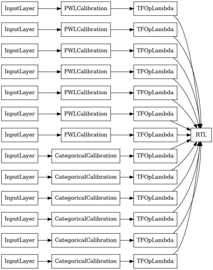
Случайный ансамбль решеток RTL Layer
При использовании решетки случайного ансамбля, вы можете указать , что модель использовать один tfl.layers.RTL слой. Отметим , что tfl.layers.RTL поддерживает только монотонности ограничения и должны иметь одинаковый размер решетки для всех функций и не за-функции упорядочению. Обратите внимание , что при использовании tfl.layers.RTL слоя позволяет масштабировать до гораздо больших ансамблей , чем при использовании отдельных tfl.layers.Lattice экземпляров.
В этом примере создается калиброванная модель ансамбля решеток с 5 решетками и 3 элементами на решетку.
# Make sure our feature configs have the same lattice size, no per-feature
# regularization, and only monotonicity constraints.
rtl_layer_feature_configs = copy.deepcopy(heart_feature_configs)
for feature_config in rtl_layer_feature_configs:
  feature_config.lattice_size = 2
  feature_config.unimodality = 'none'
  feature_config.reflects_trust_in = None
  feature_config.dominates = None
  feature_config.regularizer_configs = None
# This is a calibrated lattice ensemble model: inputs are calibrated, then
# combined non-linearly and averaged using multiple lattice layers.
rtl_layer_ensemble_model_config = tfl.configs.CalibratedLatticeEnsembleConfig(
    feature_configs=rtl_layer_feature_configs,
    lattices='rtl_layer',
    num_lattices=5,
    lattice_rank=3,
    # We initialize the output to [-2.0, 2.0] since we'll be using logits.
    output_initialization=[-2.0, 2.0],
    random_seed=42)
# A CalibratedLatticeEnsemble premade model constructed from the given
# model config. Note that we do not have to specify the lattices by calling
# a helper function (like before with random) because the RTL Layer will take
# care of that for us.
rtl_layer_ensemble_model = tfl.premade.CalibratedLatticeEnsemble(
    rtl_layer_ensemble_model_config)
# Let's plot our model.
tf.keras.utils.plot_model(
    rtl_layer_ensemble_model, show_layer_names=False, rankdir='LR')
Как и раньше, мы компилируем, подгоняем и оцениваем нашу модель.
rtl_layer_ensemble_model.compile(
    loss=tf.keras.losses.BinaryCrossentropy(from_logits=True),
    metrics=[tf.keras.metrics.AUC(from_logits=True)],
    optimizer=tf.keras.optimizers.Adam(LEARNING_RATE))
rtl_layer_ensemble_model.fit(
    heart_train_xs,
    heart_train_ys,
    epochs=NUM_EPOCHS,
    batch_size=BATCH_SIZE,
    verbose=False)
print('Test Set Evaluation...')
print(rtl_layer_ensemble_model.evaluate(heart_test_xs, heart_test_ys))
Test Set Evaluation...
2/2 [==============================] - 0s 3ms/step - loss: 0.3614 - auc_4: 0.9079
[0.36142951250076294, 0.9078947305679321]
Ансамбль кристаллической решетки
Premade также эвристический алгоритм компоновки функция, которая называется Crystals . Чтобы использовать алгоритм Crystals, сначала мы обучаем модель предварительной настройки, которая оценивает парные взаимодействия признаков. Затем мы организуем окончательный ансамбль таким образом, чтобы признаки с более нелинейными взаимодействиями находились в одних и тех же решетках.
Premade Library предлагает вспомогательные функции для создания конфигурации модели предварительной настройки и извлечения структуры кристаллов. Обратите внимание, что предварительная подгонка модели не требует полного обучения, поэтому нескольких эпох должно быть достаточно.
В этом примере создается калиброванная модель ансамбля решеток с 5 решетками и 3 элементами на решетку.
# This is a calibrated lattice ensemble model: inputs are calibrated, then
# combines non-linearly and averaged using multiple lattice layers.
crystals_ensemble_model_config = tfl.configs.CalibratedLatticeEnsembleConfig(
    feature_configs=heart_feature_configs,
    lattices='crystals',
    num_lattices=5,
    lattice_rank=3,
    # We initialize the output to [-2.0, 2.0] since we'll be using logits.
    output_initialization=[-2.0, 2.0],
    random_seed=42)
# Now that we have our model config, we can construct a prefitting model config.
prefitting_model_config = tfl.premade_lib.construct_prefitting_model_config(
    crystals_ensemble_model_config)
# A CalibratedLatticeEnsemble premade model constructed from the given
# prefitting model config.
prefitting_model = tfl.premade.CalibratedLatticeEnsemble(
    prefitting_model_config)
# We can compile and train our prefitting model as we like.
prefitting_model.compile(
    loss=tf.keras.losses.BinaryCrossentropy(from_logits=True),
    optimizer=tf.keras.optimizers.Adam(LEARNING_RATE))
prefitting_model.fit(
    heart_train_xs,
    heart_train_ys,
    epochs=PREFITTING_NUM_EPOCHS,
    batch_size=BATCH_SIZE,
    verbose=False)
# Now that we have our trained prefitting model, we can extract the crystals.
tfl.premade_lib.set_crystals_lattice_ensemble(crystals_ensemble_model_config,
                                              prefitting_model_config,
                                              prefitting_model)
# A CalibratedLatticeEnsemble premade model constructed from the given
# model config.
crystals_ensemble_model = tfl.premade.CalibratedLatticeEnsemble(
    crystals_ensemble_model_config)
# Let's plot our model.
tf.keras.utils.plot_model(
    crystals_ensemble_model, show_layer_names=False, rankdir='LR')
Как и раньше, мы компилируем, подгоняем и оцениваем нашу модель.
crystals_ensemble_model.compile(
    loss=tf.keras.losses.BinaryCrossentropy(from_logits=True),
    metrics=[tf.keras.metrics.AUC(from_logits=True)],
    optimizer=tf.keras.optimizers.Adam(LEARNING_RATE))
crystals_ensemble_model.fit(
    heart_train_xs,
    heart_train_ys,
    epochs=NUM_EPOCHS,
    batch_size=BATCH_SIZE,
    verbose=False)
print('Test Set Evaluation...')
print(crystals_ensemble_model.evaluate(heart_test_xs, heart_test_ys))
Test Set Evaluation...
2/2 [==============================] - 1s 3ms/step - loss: 0.3404 - auc_5: 0.9179
[0.34039050340652466, 0.9179198145866394]