| | |  Wyświetl źródło na GitHub Wyświetl źródło na GitHub |
JointDistributionSequential to nowo wprowadzony rozkład podobny do klasy, która pozwala użytkownikom szybko prototypowego modelu Bayesa. Pozwala łączyć ze sobą wiele dystrybucji i używać funkcji lambda do wprowadzania zależności. Jest przeznaczony do budowania małych i średnich modeli bayesowskich, w tym wielu powszechnie używanych modeli, takich jak GLM, modele z efektami mieszanymi, modele mieszane i inne. Zapewnia wszystkie niezbędne funkcje dla przepływu pracy bayesowskiej: wcześniejsze próbkowanie predykcyjne, może być podłączony do innego większego modelu graficznego bayesowskiego lub sieci neuronowej. W tym Colab, pokażemy kilka przykładów, jak używać JointDistributionSequential aby osiągnąć z dnia na dzień Bayesa workflow
Zależności i wymagania wstępne
# We will be using ArviZ, a multi-backend Bayesian diagnosis and plotting librarypip3 install -q git+git://github.com/arviz-devs/arviz.git
Importuj i konfiguruj
from pprint import pprint
import matplotlib.pyplot as plt
import numpy as np
import seaborn as sns
import pandas as pd
import arviz as az

import tensorflow.compat.v2 as tf
tf.enable_v2_behavior()

import tensorflow_probability as tfp

sns.reset_defaults()
#sns.set_style('whitegrid')
#sns.set_context('talk')
sns.set_context(context='talk',font_scale=0.7)

%config InlineBackend.figure_format = 'retina'
%matplotlib inline

tfd = tfp.distributions
tfb = tfp.bijectors

dtype = tf.float64
Zrób rzeczy szybko!
Zanim zagłębimy się w temat, upewnijmy się, że w tej wersji demonstracyjnej używamy procesora graficznego.
W tym celu wybierz „Runtime” -> „Zmień typ środowiska uruchomieniowego” -> „Hardware Accelerator” -> „GPU”.
Poniższy fragment kodu zweryfikuje, czy mamy dostęp do GPU.
if tf.test.gpu_device_name() != '/device:GPU:0':
  print('WARNING: GPU device not found.')
else:
  print('SUCCESS: Found GPU: {}'.format(tf.test.gpu_device_name()))
SUCCESS: Found GPU: /device:GPU:0
Wspólna dystrybucja
Uwagi: Ta klasa dystrybucji jest przydatna, gdy masz prosty model. „Prosty” oznacza wykresy przypominające łańcuch; chociaż podejście to technicznie działa dla każdego PGM o stopniu najwyżej 255 dla pojedynczego węzła (ponieważ funkcje Pythona mogą mieć co najwyżej tyle argumentów).
Podstawowym założeniem jest, aby użytkownik mógł określić listę callable s, które produkują tfp.Distribution instancji, po jednej dla każdego wierzchołka w ich PGM . callable będą miały co najwyżej tyle argumentów, jak jej indeksu na liście. (Dla wygody użytkownika, agumenty będą przekazywane w odwrotnej kolejności tworzenia.) Wewnętrznie „przejdziemy po wykresie”, po prostu przekazując każdą poprzednią wartość RV do każdej wywoływanej. W ten sposób możemy realizować [regułę łańcuchową prawdopodobieństwo] (https://en.wikipedia.org/wiki/Chain reguły (prawdopodobieństwo 29% # More_than_two_random_variables) \(p(\{x\}_i^d)=\prod_i^d p(x_i|x_{<i})\).
Pomysł jest dość prosty, nawet jak na kod Pythona. Oto sedno sprawy:
# The chain rule of probability, manifest as Python code.
def log_prob(rvs, xs):
  # xs[:i] is rv[i]'s markov blanket. `[::-1]` just reverses the list.
  return sum(rv(*xs[i-1::-1]).log_prob(xs[i])
             for i, rv in enumerate(rvs))
Można znaleźć więcej informacji z docstring z JointDistributionSequential , ale sens jest, aby przekazać listę dystrybucji do inicjalizacji klasy, jeśli niektóre dystrybucje na liście zależy od wyjścia z innego upstream dystrybucji / zmiennej, wystarczy owinąć go z funkcja lambda. Zobaczmy teraz, jak to działa w akcji!
(Solidny) Regresja liniowa
Od PyMC3 doc GLM: solidny regresji z wykrywaniem odstających
Otrzymać dane
dfhogg = pd.DataFrame(np.array([[1, 201, 592, 61, 9, -0.84],
[2, 244, 401, 25, 4, 0.31],
[3, 47, 583, 38, 11, 0.64],
[4, 287, 402, 15, 7, -0.27],
[5, 203, 495, 21, 5, -0.33],
[6, 58, 173, 15, 9, 0.67],
[7, 210, 479, 27, 4, -0.02],
[8, 202, 504, 14, 4, -0.05],
[9, 198, 510, 30, 11, -0.84],
[10, 158, 416, 16, 7, -0.69],
[11, 165, 393, 14, 5, 0.30],
[12, 201, 442, 25, 5, -0.46],
[13, 157, 317, 52, 5, -0.03],
[14, 131, 311, 16, 6, 0.50],
[15, 166, 400, 34, 6, 0.73],
[16, 160, 337, 31, 5, -0.52],
[17, 186, 423, 42, 9, 0.90],
[18, 125, 334, 26, 8, 0.40],
[19, 218, 533, 16, 6, -0.78],
[20, 146, 344, 22, 5, -0.56]]),
columns=['id','x','y','sigma_y','sigma_x','rho_xy'])
## for convenience zero-base the 'id' and use as index
dfhogg['id'] = dfhogg['id'] - 1
dfhogg.set_index('id', inplace=True)
## standardize (mean center and divide by 1 sd)
dfhoggs = (dfhogg[['x','y']] - dfhogg[['x','y']].mean(0)) / dfhogg[['x','y']].std(0)
dfhoggs['sigma_y'] = dfhogg['sigma_y'] / dfhogg['y'].std(0)
dfhoggs['sigma_x'] = dfhogg['sigma_x'] / dfhogg['x'].std(0)
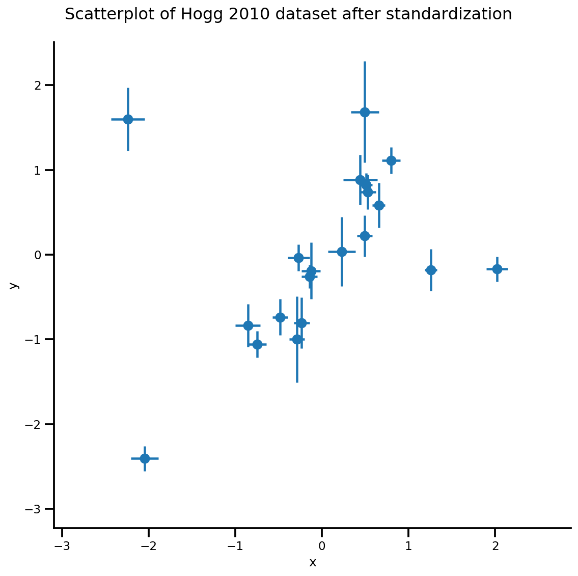
def plot_hoggs(dfhoggs):
## create xlims ylims for plotting
xlims = (dfhoggs['x'].min() - np.ptp(dfhoggs['x'])/5,
dfhoggs['x'].max() + np.ptp(dfhoggs['x'])/5)
ylims = (dfhoggs['y'].min() - np.ptp(dfhoggs['y'])/5,
dfhoggs['y'].max() + np.ptp(dfhoggs['y'])/5)
## scatterplot the standardized data
g = sns.FacetGrid(dfhoggs, size=8)
_ = g.map(plt.errorbar, 'x', 'y', 'sigma_y', 'sigma_x', marker="o", ls='')
_ = g.axes[0][0].set_ylim(ylims)
_ = g.axes[0][0].set_xlim(xlims)
plt.subplots_adjust(top=0.92)
_ = g.fig.suptitle('Scatterplot of Hogg 2010 dataset after standardization', fontsize=16)
return g, xlims, ylims
g = plot_hoggs(dfhoggs)
/usr/local/lib/python3.6/dist-packages/numpy/core/fromnumeric.py:2495: FutureWarning: Method .ptp is deprecated and will be removed in a future version. Use numpy.ptp instead.
  return ptp(axis=axis, out=out, **kwargs)
/usr/local/lib/python3.6/dist-packages/seaborn/axisgrid.py:230: UserWarning: The `size` paramter has been renamed to `height`; please update your code.
  warnings.warn(msg, UserWarning)
X_np = dfhoggs['x'].values
sigma_y_np = dfhoggs['sigma_y'].values
Y_np = dfhoggs['y'].values
Konwencjonalny model OLS
Teraz skonfigurujmy model liniowy, prosty punkt przecięcia + problem regresji nachylenia:
mdl_ols = tfd.JointDistributionSequential([
    # b0 ~ Normal(0, 1)
    tfd.Normal(loc=tf.cast(0, dtype), scale=1.),
    # b1 ~ Normal(0, 1)
    tfd.Normal(loc=tf.cast(0, dtype), scale=1.),
    # x ~ Normal(b0+b1*X, 1)
    lambda b1, b0: tfd.Normal(
      # Parameter transformation
      loc=b0 + b1*X_np,
      scale=sigma_y_np)
])
Następnie możesz sprawdzić wykres modelu, aby zobaczyć zależność. Zauważ, że x jest zarezerwowana jako nazwa ostatniego węzła, a na pewno nie można go jako argumentu lambda w swojej JointDistributionSequential modelu.
mdl_ols.resolve_graph()
(('b0', ()), ('b1', ()), ('x', ('b1', 'b0')))
Pobieranie próbek z modelu jest dość proste:
mdl_ols.sample()
[<tf.Tensor: shape=(), dtype=float64, numpy=-0.50225804634794>,
 <tf.Tensor: shape=(), dtype=float64, numpy=0.682740126293564>,
 <tf.Tensor: shape=(20,), dtype=float64, numpy=
 array([-0.33051382,  0.71443618, -1.91085683,  0.89371173, -0.45060957,
        -1.80448758, -0.21357082,  0.07891058, -0.20689721, -0.62690385,
        -0.55225748, -0.11446535, -0.66624497, -0.86913291, -0.93605552,
        -0.83965336, -0.70988597, -0.95813437,  0.15884761, -0.31113434])>]
...co daje listę tf.Tensor. Możesz od razu podłączyć go do funkcji log_prob, aby obliczyć log_prob modelu:
prior_predictive_samples = mdl_ols.sample()
mdl_ols.log_prob(prior_predictive_samples)
<tf.Tensor: shape=(20,), dtype=float64, numpy=
array([-4.97502846, -3.98544303, -4.37514505, -3.46933487, -3.80688125,
       -3.42907525, -4.03263074, -3.3646366 , -4.70370938, -4.36178501,
       -3.47823735, -3.94641662, -5.76906319, -4.0944128 , -4.39310708,
       -4.47713894, -4.46307881, -3.98802372, -3.83027747, -4.64777082])>
Hmmm, coś tu jest nie tak: powinniśmy otrzymać skalarny log_prob! W rzeczywistości, możemy dodatkowo sprawdzić, czy coś jest wyłączony przez wywołanie .log_prob_parts , co daje log_prob każdego węzłów w modelu graficznym:
mdl_ols.log_prob_parts(prior_predictive_samples)
[<tf.Tensor: shape=(), dtype=float64, numpy=-0.9699239562734849>,
 <tf.Tensor: shape=(), dtype=float64, numpy=-3.459364167569284>,
 <tf.Tensor: shape=(20,), dtype=float64, numpy=
 array([-0.54574034,  0.4438451 ,  0.05414307,  0.95995326,  0.62240687,
         1.00021288,  0.39665739,  1.06465152, -0.27442125,  0.06750311,
         0.95105078,  0.4828715 , -1.33977506,  0.33487533,  0.03618104,
        -0.04785082, -0.03379069,  0.4412644 ,  0.59901066, -0.2184827 ])>]
...okazuje się, że ostatni węzeł nie jest suma_redukcyjna wzdłuż wymiaru/osi iid! Kiedy robimy sumę, dwie pierwsze zmienne są zatem błędnie transmitowane.
Sztuką jest, aby używać tfd.Independent do reinterpretacji kształcie wsadowym (tak, że reszta osi będą zmniejszonym poprawnie):
mdl_ols_ = tfd.JointDistributionSequential([
    # b0
    tfd.Normal(loc=tf.cast(0, dtype), scale=1.),
    # b1
    tfd.Normal(loc=tf.cast(0, dtype), scale=1.),
    # likelihood
    #   Using Independent to ensure the log_prob is not incorrectly broadcasted
    lambda b1, b0: tfd.Independent(
        tfd.Normal(
            # Parameter transformation
            # b1 shape: (batch_shape), X shape (num_obs): we want result to have
            # shape (batch_shape, num_obs)
            loc=b0 + b1*X_np,
            scale=sigma_y_np),
        reinterpreted_batch_ndims=1
    ),
])
Teraz sprawdźmy ostatni węzeł/rozkład modelu, widać, że kształt zdarzenia jest teraz poprawnie interpretowany. Należy pamiętać, że może to zająć trochę prób i błędów, aby uzyskać reinterpreted_batch_ndims rację, ale zawsze można łatwo wydrukować lub dystrybucję próbkowany tensor dokładnie sprawdzić kształt!
print(mdl_ols_.sample_distributions()[0][-1])
print(mdl_ols.sample_distributions()[0][-1])
tfp.distributions.Independent("JointDistributionSequential_sample_distributions_IndependentJointDistributionSequential_sample_distributions_Normal", batch_shape=[], event_shape=[20], dtype=float64)
tfp.distributions.Normal("JointDistributionSequential_sample_distributions_Normal", batch_shape=[20], event_shape=[], dtype=float64)
prior_predictive_samples = mdl_ols_.sample()
mdl_ols_.log_prob(prior_predictive_samples)  # <== Getting a scalar correctly
<tf.Tensor: shape=(), dtype=float64, numpy=-2.543425661013286>
Inne JointDistribution* API
mdl_ols_named = tfd.JointDistributionNamed(dict(
    likelihood = lambda b0, b1: tfd.Independent(
        tfd.Normal(
            loc=b0 + b1*X_np,
            scale=sigma_y_np),
        reinterpreted_batch_ndims=1
    ),
    b0         = tfd.Normal(loc=tf.cast(0, dtype), scale=1.),
    b1         = tfd.Normal(loc=tf.cast(0, dtype), scale=1.),
))

mdl_ols_named.log_prob(mdl_ols_named.sample())
<tf.Tensor: shape=(), dtype=float64, numpy=-5.99620966071338>
mdl_ols_named.sample() # output is a dictionary
{'b0': <tf.Tensor: shape=(), dtype=float64, numpy=0.26364058399428225>,
 'b1': <tf.Tensor: shape=(), dtype=float64, numpy=-0.27209402374432207>,
 'likelihood': <tf.Tensor: shape=(20,), dtype=float64, numpy=
 array([ 0.6482155 , -0.39314108,  0.62744764, -0.24587987, -0.20544617,
         1.01465392, -0.04705611, -0.16618702,  0.36410134,  0.3943299 ,
         0.36455291, -0.27822219, -0.24423928,  0.24599518,  0.82731092,
        -0.21983033,  0.56753169,  0.32830481, -0.15713064,  0.23336351])>}
Root = tfd.JointDistributionCoroutine.Root  # Convenient alias.
def model():
  b1 = yield Root(tfd.Normal(loc=tf.cast(0, dtype), scale=1.))
  b0 = yield Root(tfd.Normal(loc=tf.cast(0, dtype), scale=1.))
  yhat = b0 + b1*X_np
  likelihood = yield tfd.Independent(
        tfd.Normal(loc=yhat, scale=sigma_y_np),
        reinterpreted_batch_ndims=1
    )

mdl_ols_coroutine = tfd.JointDistributionCoroutine(model)
mdl_ols_coroutine.log_prob(mdl_ols_coroutine.sample())
<tf.Tensor: shape=(), dtype=float64, numpy=-4.566678123520463>
mdl_ols_coroutine.sample() # output is a tuple
(<tf.Tensor: shape=(), dtype=float64, numpy=0.06811002171170354>,
 <tf.Tensor: shape=(), dtype=float64, numpy=-0.37477064754116807>,
 <tf.Tensor: shape=(20,), dtype=float64, numpy=
 array([-0.91615096, -0.20244718, -0.47840159, -0.26632479, -0.60441105,
        -0.48977789, -0.32422329, -0.44019322, -0.17072643, -0.20666025,
        -0.55932191, -0.40801868, -0.66893181, -0.24134135, -0.50403536,
        -0.51788596, -0.90071876, -0.47382338, -0.34821655, -0.38559724])>)
MLE
A teraz możemy wnioskować! Możesz użyć optymalizatora, aby znaleźć oszacowanie maksymalnego prawdopodobieństwa.
Zdefiniuj niektóre funkcje pomocnicze
# bfgs and lbfgs currently requries a function that returns both the value and
# gradient re the input.
import functools

def _make_val_and_grad_fn(value_fn):
  @functools.wraps(value_fn)
  def val_and_grad(x):
    return tfp.math.value_and_gradient(value_fn, x)
  return val_and_grad

# Map a list of tensors (e.g., output from JDSeq.sample([...])) to a single tensor
# modify from tfd.Blockwise
from tensorflow_probability.python.internal import dtype_util
from tensorflow_probability.python.internal import prefer_static as ps
from tensorflow_probability.python.internal import tensorshape_util

class Mapper:
  """Basically, this is a bijector without log-jacobian correction."""
  def __init__(self, list_of_tensors, list_of_bijectors, event_shape):
    self.dtype = dtype_util.common_dtype(
        list_of_tensors, dtype_hint=tf.float32)
    self.list_of_tensors = list_of_tensors
    self.bijectors = list_of_bijectors
    self.event_shape = event_shape

  def flatten_and_concat(self, list_of_tensors):
    def _reshape_map_part(part, event_shape, bijector):
      part = tf.cast(bijector.inverse(part), self.dtype)
      static_rank = tf.get_static_value(ps.rank_from_shape(event_shape))
      if static_rank == 1:
        return part
      new_shape = ps.concat([
          ps.shape(part)[:ps.size(ps.shape(part)) - ps.size(event_shape)],
          [-1]
      ], axis=-1)
      return tf.reshape(part, ps.cast(new_shape, tf.int32))

    x = tf.nest.map_structure(_reshape_map_part,
                              list_of_tensors,
                              self.event_shape,
                              self.bijectors)
    return tf.concat(tf.nest.flatten(x), axis=-1)

  def split_and_reshape(self, x):
    assertions = []
    message = 'Input must have at least one dimension.'
    if tensorshape_util.rank(x.shape) is not None:
      if tensorshape_util.rank(x.shape) == 0:
        raise ValueError(message)
    else:
      assertions.append(assert_util.assert_rank_at_least(x, 1, message=message))
    with tf.control_dependencies(assertions):
      splits = [
          tf.cast(ps.maximum(1, ps.reduce_prod(s)), tf.int32)
          for s in tf.nest.flatten(self.event_shape)
      ]
      x = tf.nest.pack_sequence_as(
          self.event_shape, tf.split(x, splits, axis=-1))
      def _reshape_map_part(part, part_org, event_shape, bijector):
        part = tf.cast(bijector.forward(part), part_org.dtype)
        static_rank = tf.get_static_value(ps.rank_from_shape(event_shape))
        if static_rank == 1:
          return part
        new_shape = ps.concat([ps.shape(part)[:-1], event_shape], axis=-1)
        return tf.reshape(part, ps.cast(new_shape, tf.int32))

      x = tf.nest.map_structure(_reshape_map_part,
                                x,
                                self.list_of_tensors,
                                self.event_shape,
                                self.bijectors)
    return x
mapper = Mapper(mdl_ols_.sample()[:-1],
                [tfb.Identity(), tfb.Identity()],
                mdl_ols_.event_shape[:-1])

# mapper.split_and_reshape(mapper.flatten_and_concat(mdl_ols_.sample()[:-1]))
@_make_val_and_grad_fn
def neg_log_likelihood(x):
  # Generate a function closure so that we are computing the log_prob
  # conditioned on the observed data. Note also that tfp.optimizer.* takes a
  # single tensor as input.
  return -mdl_ols_.log_prob(mapper.split_and_reshape(x) + [Y_np])

lbfgs_results = tfp.optimizer.lbfgs_minimize(
    neg_log_likelihood,
    initial_position=tf.zeros(2, dtype=dtype),
    tolerance=1e-20,
    x_tolerance=1e-8
)
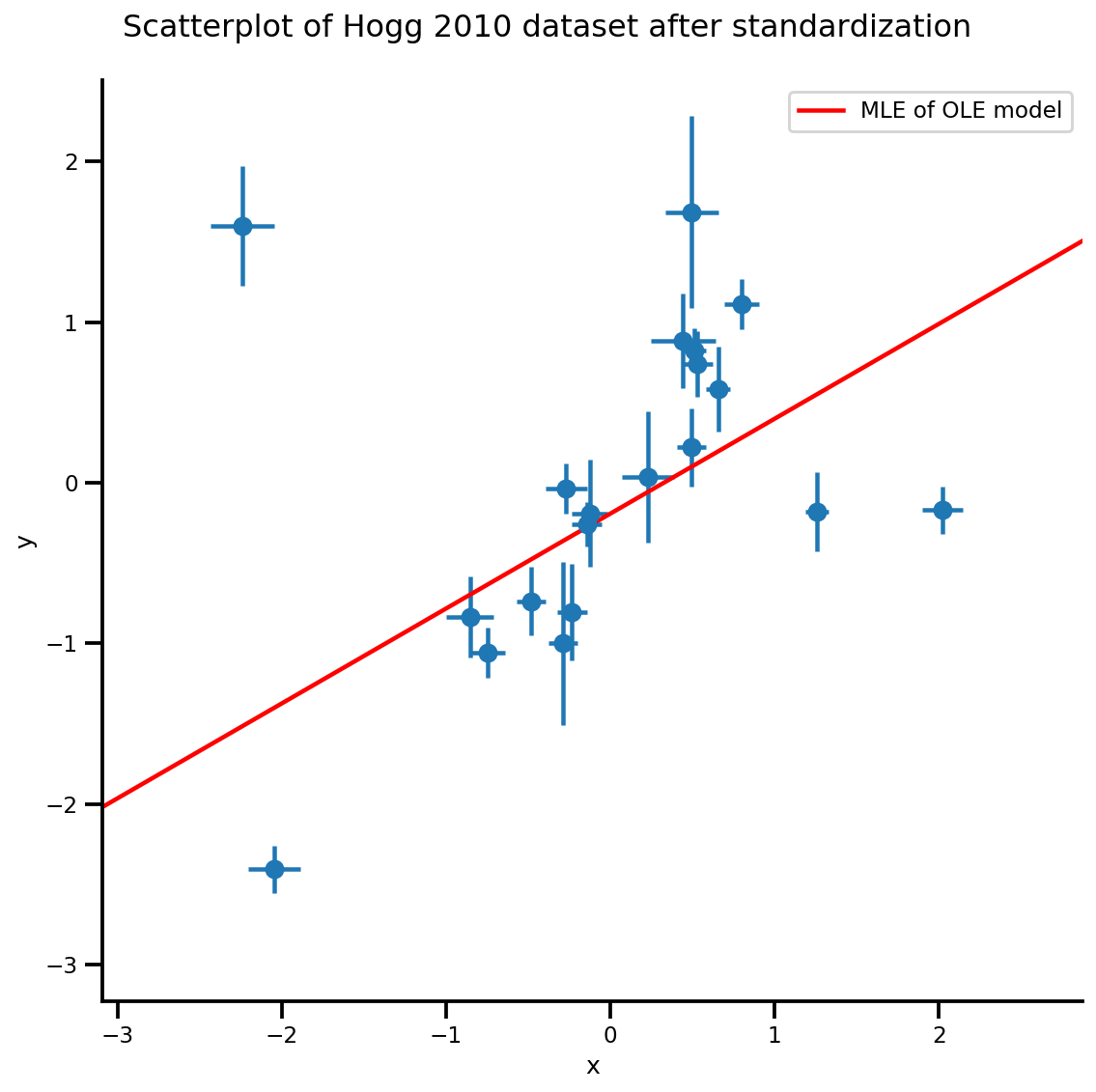
b0est, b1est = lbfgs_results.position.numpy()

g, xlims, ylims = plot_hoggs(dfhoggs);
xrange = np.linspace(xlims[0], xlims[1], 100)
g.axes[0][0].plot(xrange, b0est + b1est*xrange,
                  color='r', label='MLE of OLE model')
plt.legend();
/usr/local/lib/python3.6/dist-packages/numpy/core/fromnumeric.py:2495: FutureWarning: Method .ptp is deprecated and will be removed in a future version. Use numpy.ptp instead.
  return ptp(axis=axis, out=out, **kwargs)
/usr/local/lib/python3.6/dist-packages/seaborn/axisgrid.py:230: UserWarning: The `size` paramter has been renamed to `height`; please update your code.
  warnings.warn(msg, UserWarning)
Model wersji wsadowej i MCMC
W Bayesa Inference, zwykle chcą pracować z próbkami MCMC, jak wtedy, gdy próbki są od tylnej, możemy podłączyć do dowolnej funkcji do obliczania oczekiwań. Jednak MCMC API wymagają od nas napisać modele, które są przyjazne dla partii, a my możemy sprawdzić, że nasz model jest rzeczywiście nie „batchable” wywołując sample([...])
mdl_ols_.sample(5) # <== error as some computation could not be broadcasted.
W tym przypadku jest to stosunkowo proste, ponieważ w naszym modelu mamy tylko funkcję liniową, rozszerzenie kształtu powinno wystarczyć:
mdl_ols_batch = tfd.JointDistributionSequential([
    # b0
    tfd.Normal(loc=tf.cast(0, dtype), scale=1.),
    # b1
    tfd.Normal(loc=tf.cast(0, dtype), scale=1.),
    # likelihood
    #   Using Independent to ensure the log_prob is not incorrectly broadcasted
    lambda b1, b0: tfd.Independent(
        tfd.Normal(
            # Parameter transformation
            loc=b0[..., tf.newaxis] + b1[..., tf.newaxis]*X_np[tf.newaxis, ...],
            scale=sigma_y_np[tf.newaxis, ...]),
        reinterpreted_batch_ndims=1
    ),
])

mdl_ols_batch.resolve_graph()
(('b0', ()), ('b1', ()), ('x', ('b1', 'b0')))
Możemy ponownie pobrać próbkę i ocenić log_prob_parts, aby wykonać kilka sprawdzeń:
b0, b1, y = mdl_ols_batch.sample(4)
mdl_ols_batch.log_prob_parts([b0, b1, y])
[<tf.Tensor: shape=(4,), dtype=float64, numpy=array([-1.25230168, -1.45281432, -1.87110061, -1.07665206])>,
 <tf.Tensor: shape=(4,), dtype=float64, numpy=array([-1.07019936, -1.59562117, -2.53387765, -1.01557632])>,
 <tf.Tensor: shape=(4,), dtype=float64, numpy=array([ 0.45841406,  2.56829635, -4.84973951, -5.59423992])>]
Kilka uwag pobocznych:
- Chcemy pracować z wsadową wersją modelu, ponieważ jest to najszybsze rozwiązanie dla wielołańcuchowych MCMC. W przypadkach, których nie można przepisać model jako dozowanego wersji (np modele ODE), można odwzorować za pomocą funkcji log_prob
tf.map_fnaby osiągnąć ten sam efekt. - Teraz
mdl_ols_batch.sample()może nie działać jak mamy skaler przed, jak nie możemy zrobićscaler_tensor[:, None]. Rozwiązaniem tego problemu jest zwiększenie skalowania tensor Rank 1 owijająctfd.Sample(..., sample_shape=1). - Dobrą praktyką jest napisanie modelu jako funkcji, dzięki czemu można znacznie łatwiej zmieniać ustawienia, takie jak hiperparametry.
def gen_ols_batch_model(X, sigma, hyperprior_mean=0, hyperprior_scale=1):
  hyper_mean = tf.cast(hyperprior_mean, dtype)
  hyper_scale = tf.cast(hyperprior_scale, dtype)
  return tfd.JointDistributionSequential([
      # b0
      tfd.Sample(tfd.Normal(loc=hyper_mean, scale=hyper_scale), sample_shape=1),
      # b1
      tfd.Sample(tfd.Normal(loc=hyper_mean, scale=hyper_scale), sample_shape=1),
      # likelihood
      lambda b1, b0: tfd.Independent(
          tfd.Normal(
              # Parameter transformation
              loc=b0 + b1*X,
              scale=sigma),
          reinterpreted_batch_ndims=1
      ),
  ], validate_args=True)

mdl_ols_batch = gen_ols_batch_model(X_np[tf.newaxis, ...],
                                    sigma_y_np[tf.newaxis, ...])

_ = mdl_ols_batch.sample()
_ = mdl_ols_batch.sample(4)
_ = mdl_ols_batch.sample([3, 4])
# Small helper function to validate log_prob shape (avoid wrong broadcasting)
def validate_log_prob_part(model, batch_shape=1, observed=-1):
  samples = model.sample(batch_shape)
  logp_part = list(model.log_prob_parts(samples))

  # exclude observed node
  logp_part.pop(observed)
  for part in logp_part:
    tf.assert_equal(part.shape, logp_part[-1].shape)

validate_log_prob_part(mdl_ols_batch, 4)
Więcej sprawdzeń: porównanie wygenerowanej funkcji log_prob z ręcznie napisaną funkcją log_prob TFP.
def ols_logp_batch(b0, b1, Y):
  b0_prior = tfd.Normal(loc=tf.cast(0, dtype), scale=1.) # b0
  b1_prior = tfd.Normal(loc=tf.cast(0, dtype), scale=1.) # b1
  likelihood = tfd.Normal(loc=b0 + b1*X_np[None, :],
                          scale=sigma_y_np) # likelihood
  return tf.reduce_sum(b0_prior.log_prob(b0), axis=-1) +\
         tf.reduce_sum(b1_prior.log_prob(b1), axis=-1) +\
         tf.reduce_sum(likelihood.log_prob(Y), axis=-1)

b0, b1, x = mdl_ols_batch.sample(4)
print(mdl_ols_batch.log_prob([b0, b1, Y_np]).numpy())
print(ols_logp_batch(b0, b1, Y_np).numpy())
[-227.37899384 -327.10043743 -570.44162789 -702.79808683]
[-227.37899384 -327.10043743 -570.44162789 -702.79808683]
MCMC przy użyciu próbnika bez zawracania
Częstym run_chain funkcja
@tf.function(autograph=False, experimental_compile=True)
def run_chain(init_state, step_size, target_log_prob_fn, unconstraining_bijectors,
              num_steps=500, burnin=50):

  def trace_fn(_, pkr):
    return (
        pkr.inner_results.inner_results.target_log_prob,
        pkr.inner_results.inner_results.leapfrogs_taken,
        pkr.inner_results.inner_results.has_divergence,
        pkr.inner_results.inner_results.energy,
        pkr.inner_results.inner_results.log_accept_ratio
           )

  kernel = tfp.mcmc.TransformedTransitionKernel(
    inner_kernel=tfp.mcmc.NoUTurnSampler(
      target_log_prob_fn,
      step_size=step_size),
    bijector=unconstraining_bijectors)

  hmc = tfp.mcmc.DualAveragingStepSizeAdaptation(
    inner_kernel=kernel,
    num_adaptation_steps=burnin,
    step_size_setter_fn=lambda pkr, new_step_size: pkr._replace(
        inner_results=pkr.inner_results._replace(step_size=new_step_size)),
    step_size_getter_fn=lambda pkr: pkr.inner_results.step_size,
    log_accept_prob_getter_fn=lambda pkr: pkr.inner_results.log_accept_ratio
  )

  # Sampling from the chain.
  chain_state, sampler_stat = tfp.mcmc.sample_chain(
      num_results=num_steps,
      num_burnin_steps=burnin,
      current_state=init_state,
      kernel=hmc,
      trace_fn=trace_fn)
  return chain_state, sampler_stat
nchain = 10
b0, b1, _ = mdl_ols_batch.sample(nchain)
init_state = [b0, b1]
step_size = [tf.cast(i, dtype=dtype) for i in [.1, .1]]
target_log_prob_fn = lambda *x: mdl_ols_batch.log_prob(x + (Y_np, ))

# bijector to map contrained parameters to real
unconstraining_bijectors = [
    tfb.Identity(),
    tfb.Identity(),
]

samples, sampler_stat = run_chain(
    init_state, step_size, target_log_prob_fn, unconstraining_bijectors)
# using the pymc3 naming convention
sample_stats_name = ['lp', 'tree_size', 'diverging', 'energy', 'mean_tree_accept']
sample_stats = {k:v.numpy().T for k, v in zip(sample_stats_name, sampler_stat)}
sample_stats['tree_size'] = np.diff(sample_stats['tree_size'], axis=1)
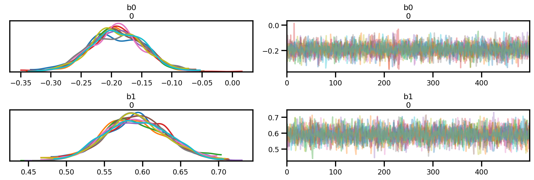
var_name = ['b0', 'b1']
posterior = {k:np.swapaxes(v.numpy(), 1, 0)
for k, v in zip(var_name, samples)}
az_trace = az.from_dict(posterior=posterior, sample_stats=sample_stats)
az.plot_trace(az_trace);
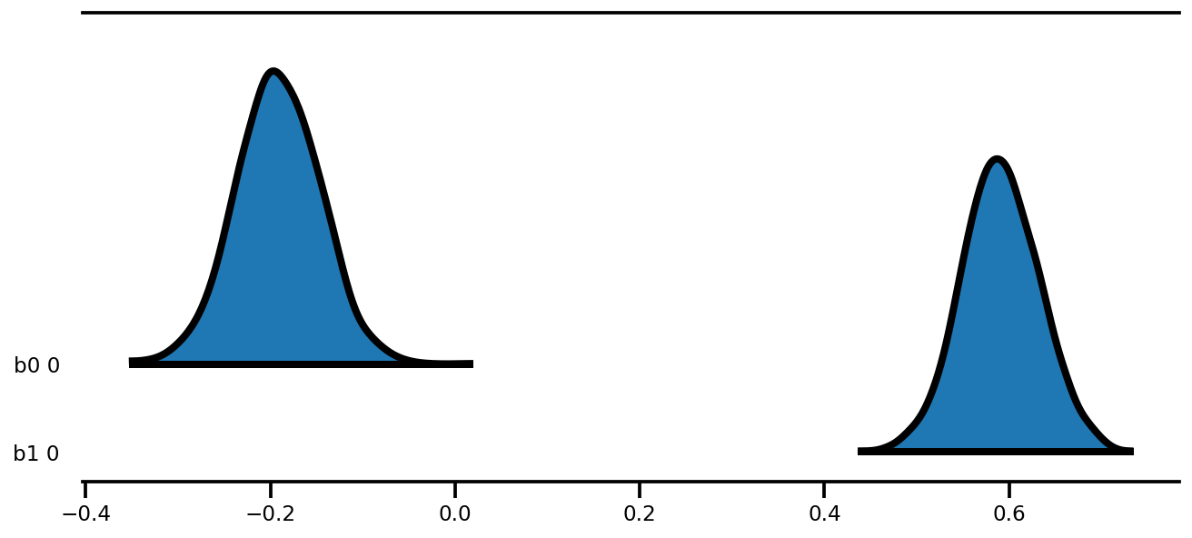
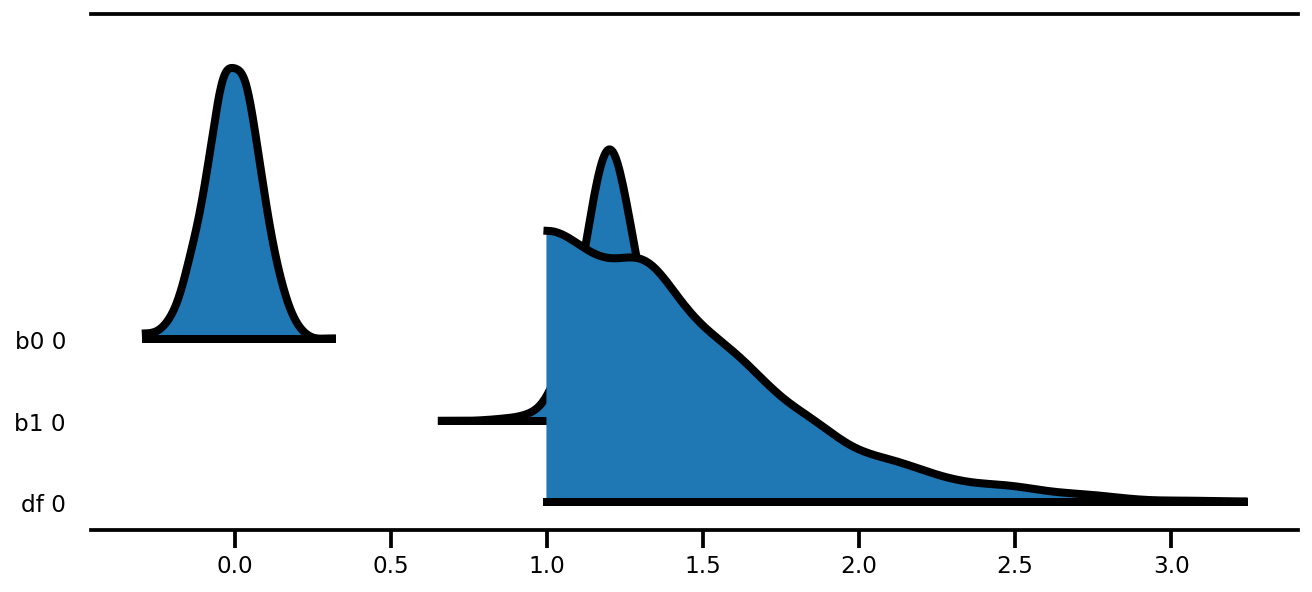
az.plot_forest(az_trace,
               kind='ridgeplot',
               linewidth=4,
               combined=True,
               ridgeplot_overlap=1.5,
               figsize=(9, 4));
k = 5
b0est, b1est = az_trace.posterior['b0'][:, -k:].values, az_trace.posterior['b1'][:, -k:].values
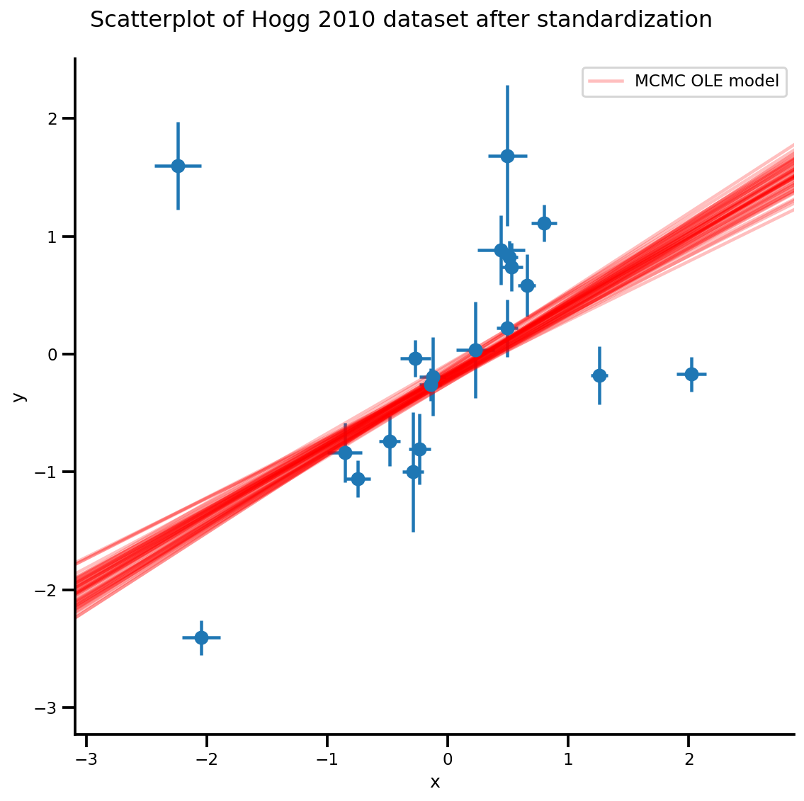
g, xlims, ylims = plot_hoggs(dfhoggs);
xrange = np.linspace(xlims[0], xlims[1], 100)[None, :]
g.axes[0][0].plot(np.tile(xrange, (k, 1)).T,
(np.reshape(b0est, [-1, 1]) + np.reshape(b1est, [-1, 1])*xrange).T,
alpha=.25, color='r')
plt.legend([g.axes[0][0].lines[-1]], ['MCMC OLE model']);
/usr/local/lib/python3.6/dist-packages/numpy/core/fromnumeric.py:2495: FutureWarning: Method .ptp is deprecated and will be removed in a future version. Use numpy.ptp instead.
  return ptp(axis=axis, out=out, **kwargs)
/usr/local/lib/python3.6/dist-packages/seaborn/axisgrid.py:230: UserWarning: The `size` paramter has been renamed to `height`; please update your code.
  warnings.warn(msg, UserWarning)
/usr/local/lib/python3.6/dist-packages/ipykernel_launcher.py:8: MatplotlibDeprecationWarning: cycling among columns of inputs with non-matching shapes is deprecated.
Metoda Studenta-T
Pamiętaj, że od teraz zawsze pracujemy z wersją wsadową modelu
def gen_studentt_model(X, sigma,
                       hyper_mean=0, hyper_scale=1, lower=1, upper=100):
  loc = tf.cast(hyper_mean, dtype)
  scale = tf.cast(hyper_scale, dtype)
  low = tf.cast(lower, dtype)
  high = tf.cast(upper, dtype)
  return tfd.JointDistributionSequential([
      # b0 ~ Normal(0, 1)
      tfd.Sample(tfd.Normal(loc, scale), sample_shape=1),
      # b1 ~ Normal(0, 1)
      tfd.Sample(tfd.Normal(loc, scale), sample_shape=1),
      # df ~ Uniform(a, b)
      tfd.Sample(tfd.Uniform(low, high), sample_shape=1),
      # likelihood ~ StudentT(df, f(b0, b1), sigma_y)
      #   Using Independent to ensure the log_prob is not incorrectly broadcasted.
      lambda df, b1, b0: tfd.Independent(
          tfd.StudentT(df=df, loc=b0 + b1*X, scale=sigma)),
  ], validate_args=True)

mdl_studentt = gen_studentt_model(X_np[tf.newaxis, ...],
                                  sigma_y_np[tf.newaxis, ...])
mdl_studentt.resolve_graph()
(('b0', ()), ('b1', ()), ('df', ()), ('x', ('df', 'b1', 'b0')))
validate_log_prob_part(mdl_studentt, 4)
Próbka do przodu (uprzednie próbkowanie predykcyjne)
b0, b1, df, x = mdl_studentt.sample(1000)
x.shape
TensorShape([1000, 20])
MLE
# bijector to map contrained parameters to real
a, b = tf.constant(1., dtype), tf.constant(100., dtype),

# Interval transformation
tfp_interval = tfb.Inline(
    inverse_fn=(
        lambda x: tf.math.log(x - a) - tf.math.log(b - x)),
    forward_fn=(
        lambda y: (b - a) * tf.sigmoid(y) + a),
    forward_log_det_jacobian_fn=(
        lambda x: tf.math.log(b - a) - 2 * tf.nn.softplus(-x) - x),
    forward_min_event_ndims=0,
    name="interval")

unconstraining_bijectors = [
    tfb.Identity(),
    tfb.Identity(),
    tfp_interval,
]

mapper = Mapper(mdl_studentt.sample()[:-1],
                unconstraining_bijectors,
                mdl_studentt.event_shape[:-1])
@_make_val_and_grad_fn
def neg_log_likelihood(x):
  # Generate a function closure so that we are computing the log_prob
  # conditioned on the observed data. Note also that tfp.optimizer.* takes a
  # single tensor as input, so we need to do some slicing here:
  return -tf.squeeze(mdl_studentt.log_prob(
      mapper.split_and_reshape(x) + [Y_np]))

lbfgs_results = tfp.optimizer.lbfgs_minimize(
    neg_log_likelihood,
    initial_position=mapper.flatten_and_concat(mdl_studentt.sample()[:-1]),
    tolerance=1e-20,
    x_tolerance=1e-20
)
b0est, b1est, dfest = lbfgs_results.position.numpy()
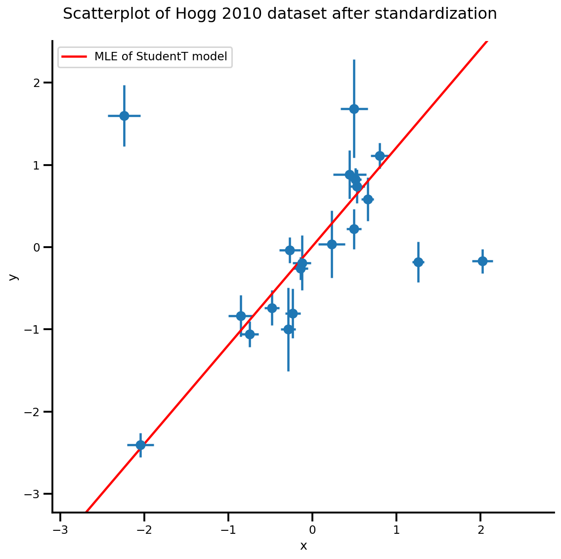
g, xlims, ylims = plot_hoggs(dfhoggs);
xrange = np.linspace(xlims[0], xlims[1], 100)
g.axes[0][0].plot(xrange, b0est + b1est*xrange,
color='r', label='MLE of StudentT model')
plt.legend();
/usr/local/lib/python3.6/dist-packages/numpy/core/fromnumeric.py:2495: FutureWarning: Method .ptp is deprecated and will be removed in a future version. Use numpy.ptp instead.
  return ptp(axis=axis, out=out, **kwargs)
/usr/local/lib/python3.6/dist-packages/seaborn/axisgrid.py:230: UserWarning: The `size` paramter has been renamed to `height`; please update your code.
  warnings.warn(msg, UserWarning)
MCMC
nchain = 10
b0, b1, df, _ = mdl_studentt.sample(nchain)
init_state = [b0, b1, df]
step_size = [tf.cast(i, dtype=dtype) for i in [.1, .1, .05]]

target_log_prob_fn = lambda *x: mdl_studentt.log_prob(x + (Y_np, ))

samples, sampler_stat = run_chain(
    init_state, step_size, target_log_prob_fn, unconstraining_bijectors, burnin=100)
# using the pymc3 naming convention
sample_stats_name = ['lp', 'tree_size', 'diverging', 'energy', 'mean_tree_accept']
sample_stats = {k:v.numpy().T for k, v in zip(sample_stats_name, sampler_stat)}
sample_stats['tree_size'] = np.diff(sample_stats['tree_size'], axis=1)

var_name = ['b0', 'b1', 'df']
posterior = {k:np.swapaxes(v.numpy(), 1, 0)
             for k, v in zip(var_name, samples)}

az_trace = az.from_dict(posterior=posterior, sample_stats=sample_stats)
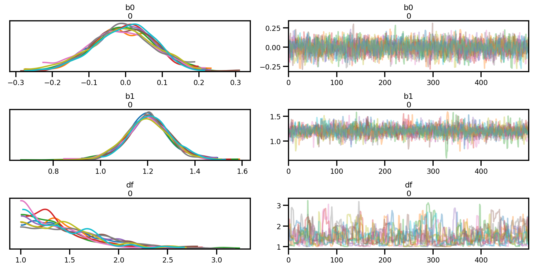
az.summary(az_trace)
az.plot_trace(az_trace);
az.plot_forest(az_trace,
               kind='ridgeplot',
               linewidth=4,
               combined=True,
               ridgeplot_overlap=1.5,
               figsize=(9, 4));
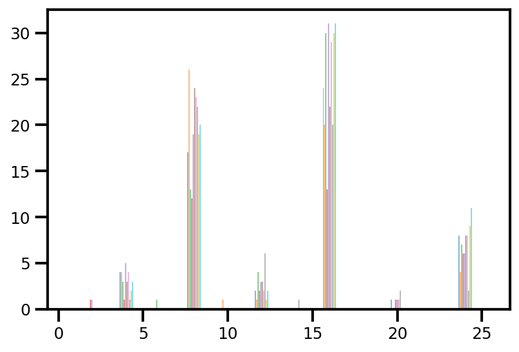
plt.hist(az_trace.sample_stats['tree_size'], np.linspace(.5, 25.5, 26), alpha=.5);
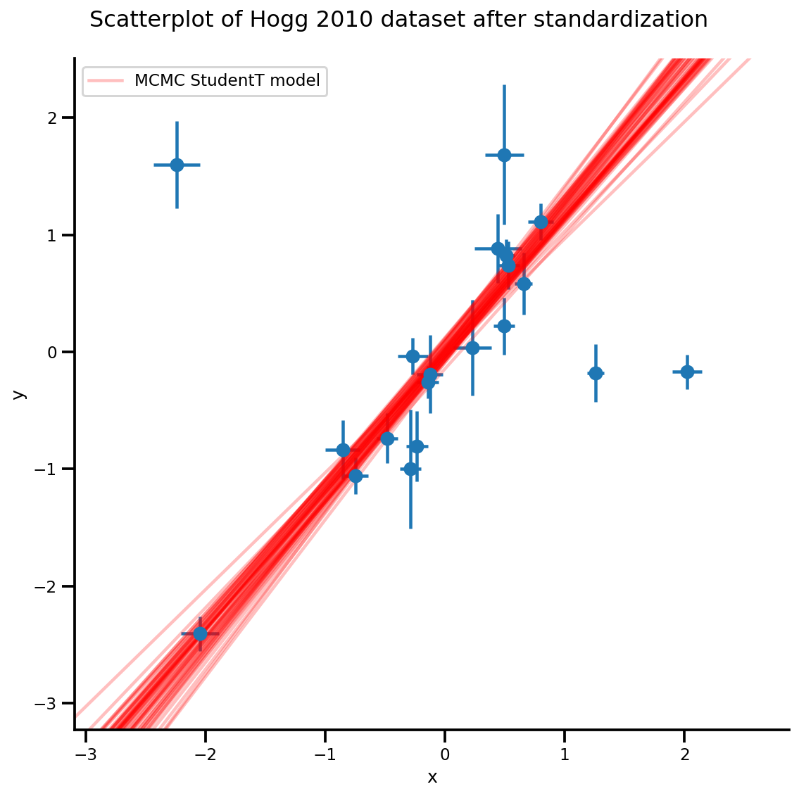
k = 5
b0est, b1est = az_trace.posterior['b0'][:, -k:].values, az_trace.posterior['b1'][:, -k:].values

g, xlims, ylims = plot_hoggs(dfhoggs);
xrange = np.linspace(xlims[0], xlims[1], 100)[None, :]
g.axes[0][0].plot(np.tile(xrange, (k, 1)).T,
                  (np.reshape(b0est, [-1, 1]) + np.reshape(b1est, [-1, 1])*xrange).T,
                  alpha=.25, color='r')
plt.legend([g.axes[0][0].lines[-1]], ['MCMC StudentT model']);
/usr/local/lib/python3.6/dist-packages/numpy/core/fromnumeric.py:2495: FutureWarning: Method .ptp is deprecated and will be removed in a future version. Use numpy.ptp instead.
  return ptp(axis=axis, out=out, **kwargs)
/usr/local/lib/python3.6/dist-packages/seaborn/axisgrid.py:230: UserWarning: The `size` paramter has been renamed to `height`; please update your code.
  warnings.warn(msg, UserWarning)
/usr/local/lib/python3.6/dist-packages/ipykernel_launcher.py:8: MatplotlibDeprecationWarning: cycling among columns of inputs with non-matching shapes is deprecated.
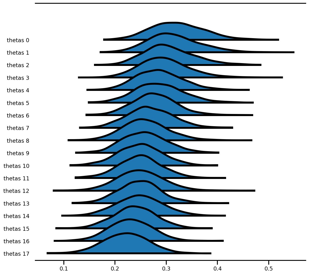
Hierarchiczne łączenie częściowe
Od PyMC3 danych z daszkiem dla 18 graczy z Efron i Morris (1975)
data = pd.read_table('https://raw.githubusercontent.com/pymc-devs/pymc3/master/pymc3/examples/data/efron-morris-75-data.tsv',
                     sep="\t")
at_bats, hits = data[['At-Bats', 'Hits']].values.T
n = len(at_bats)
def gen_baseball_model(at_bats, rate=1.5, a=0, b=1):
  return tfd.JointDistributionSequential([
    # phi
    tfd.Uniform(low=tf.cast(a, dtype), high=tf.cast(b, dtype)),
    # kappa_log
    tfd.Exponential(rate=tf.cast(rate, dtype)),
    # thetas
    lambda kappa_log, phi: tfd.Sample(
        tfd.Beta(
            concentration1=tf.exp(kappa_log)*phi,
            concentration0=tf.exp(kappa_log)*(1.0-phi)),
        sample_shape=n
    ),
    # likelihood
    lambda thetas: tfd.Independent(
        tfd.Binomial(
            total_count=tf.cast(at_bats, dtype),
            probs=thetas
        )),
])

mdl_baseball = gen_baseball_model(at_bats)
mdl_baseball.resolve_graph()
(('phi', ()),
 ('kappa_log', ()),
 ('thetas', ('kappa_log', 'phi')),
 ('x', ('thetas',)))
Próbka do przodu (uprzednie próbkowanie predykcyjne)
phi, kappa_log, thetas, y = mdl_baseball.sample(4)
# phi, kappa_log, thetas, y
Znowu zauważ, że jeśli nie użyjesz Independent, otrzymasz log_prob, który ma zły kształt wsadowy.
# check logp
pprint(mdl_baseball.log_prob_parts([phi, kappa_log, thetas, hits]))
print(mdl_baseball.log_prob([phi, kappa_log, thetas, hits]))
[<tf.Tensor: shape=(4,), dtype=float64, numpy=array([0., 0., 0., 0.])>,
 <tf.Tensor: shape=(4,), dtype=float64, numpy=array([ 0.1721297 , -0.95946498, -0.72591188,  0.23993813])>,
 <tf.Tensor: shape=(4,), dtype=float64, numpy=array([59.35192283,  7.0650634 ,  0.83744911, 74.14370935])>,
 <tf.Tensor: shape=(4,), dtype=float64, numpy=array([-3279.75191016,  -931.10438484,  -512.59197688, -1131.08043597])>]
tf.Tensor([-3220.22785762  -924.99878641  -512.48043966 -1056.69678849], shape=(4,), dtype=float64)
MLE
Całkiem niesamowite cechą tfp.optimizer jest to, że można zoptymalizowany równolegle do k partii punkt początkowy i określić stopping_condition kwarg: można ustawić go tfp.optimizer.converged_all aby sprawdzić, czy wszystkie one znaleźć takie same minimalne, lub tfp.optimizer.converged_any znaleźć lokalnego rozwiązania szybko.
unconstraining_bijectors = [
    tfb.Sigmoid(),
    tfb.Exp(),
    tfb.Sigmoid(),
]

phi, kappa_log, thetas, y = mdl_baseball.sample(10)

mapper = Mapper([phi, kappa_log, thetas],
                unconstraining_bijectors,
                mdl_baseball.event_shape[:-1])
@_make_val_and_grad_fn
def neg_log_likelihood(x):
  return -mdl_baseball.log_prob(mapper.split_and_reshape(x) + [hits])

start = mapper.flatten_and_concat([phi, kappa_log, thetas])

lbfgs_results = tfp.optimizer.lbfgs_minimize(
    neg_log_likelihood,
    num_correction_pairs=10,
    initial_position=start,
    # lbfgs actually can work in batch as well
    stopping_condition=tfp.optimizer.converged_any,
    tolerance=1e-50,
    x_tolerance=1e-50,
    parallel_iterations=10,
    max_iterations=200
)
lbfgs_results.converged.numpy(), lbfgs_results.failed.numpy()
(array([False, False, False, False, False, False, False, False, False,
        False]),
 array([ True,  True,  True,  True,  True,  True,  True,  True,  True,
         True]))
result = lbfgs_results.position[lbfgs_results.converged & ~lbfgs_results.failed]
result
<tf.Tensor: shape=(0, 20), dtype=float64, numpy=array([], shape=(0, 20), dtype=float64)>
LBFGS nie zbiegły się.
if result.shape[0] > 0:
  phi_est, kappa_est, theta_est = mapper.split_and_reshape(result)
  phi_est, kappa_est, theta_est
MCMC
target_log_prob_fn = lambda *x: mdl_baseball.log_prob(x + (hits, ))

nchain = 4
phi, kappa_log, thetas, _ = mdl_baseball.sample(nchain)
init_state = [phi, kappa_log, thetas]
step_size=[tf.cast(i, dtype=dtype) for i in [.1, .1, .1]]

samples, sampler_stat = run_chain(
    init_state, step_size, target_log_prob_fn, unconstraining_bijectors,
    burnin=200)
# using the pymc3 naming convention
sample_stats_name = ['lp', 'tree_size', 'diverging', 'energy', 'mean_tree_accept']
sample_stats = {k:v.numpy().T for k, v in zip(sample_stats_name, sampler_stat)}
sample_stats['tree_size'] = np.diff(sample_stats['tree_size'], axis=1)

var_name = ['phi', 'kappa_log', 'thetas']
posterior = {k:np.swapaxes(v.numpy(), 1, 0)
             for k, v in zip(var_name, samples)}

az_trace = az.from_dict(posterior=posterior, sample_stats=sample_stats)
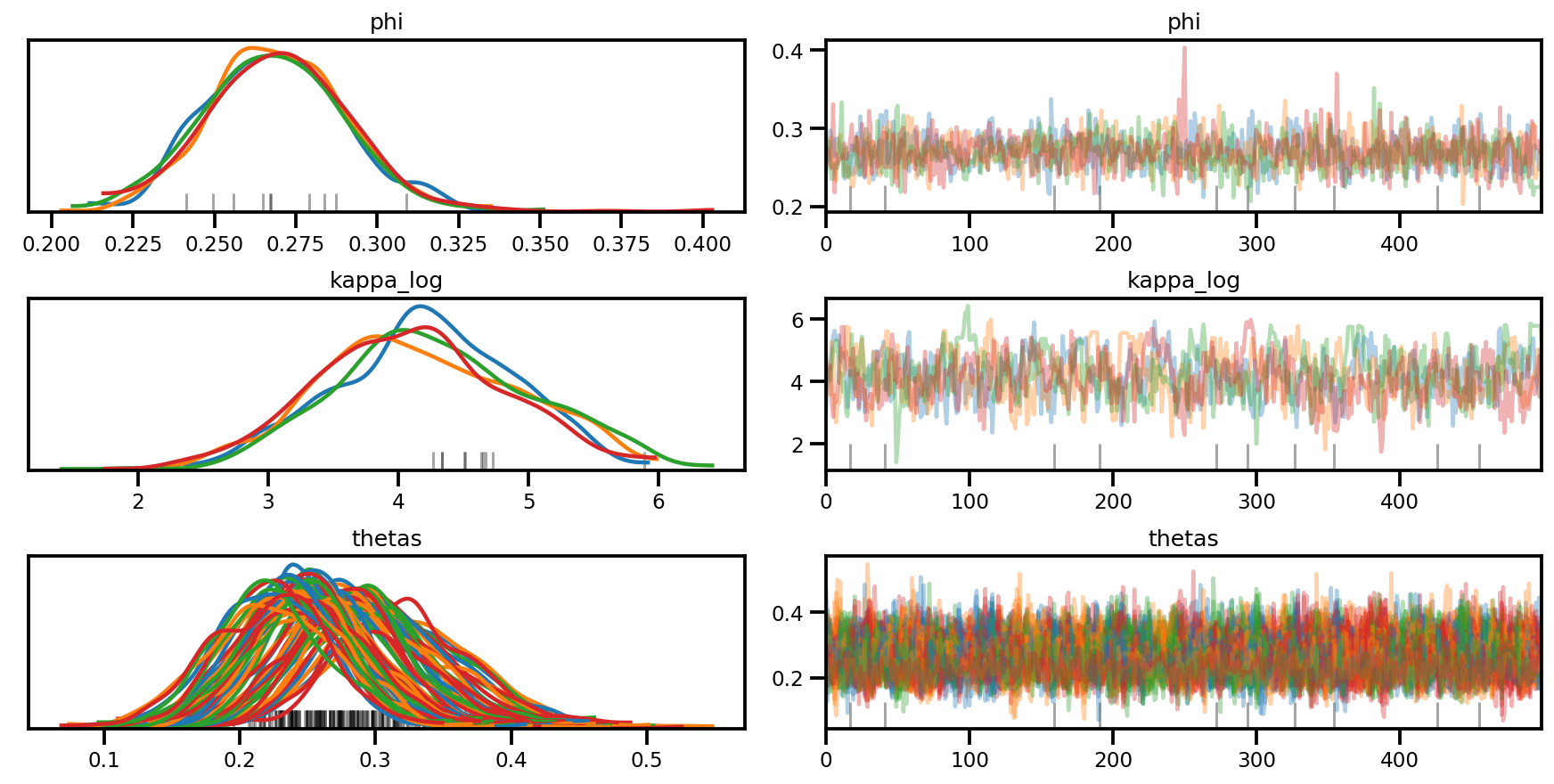
az.plot_trace(az_trace, compact=True);
az.plot_forest(az_trace,
               var_names=['thetas'],
               kind='ridgeplot',
               linewidth=4,
               combined=True,
               ridgeplot_overlap=1.5,
               figsize=(9, 8));
Model z efektem mieszanym (Radon)
Ostatnim modelem w doc PyMC3: Primer na Bayesa Metody modelowania wielopoziomowego
Niektóre zmiany w przeszłości (mniejsza skala itp.)
Załaduj surowe dane i wyczyść
srrs2 = pd.read_csv('https://raw.githubusercontent.com/pymc-devs/pymc3/master/pymc3/examples/data/srrs2.dat')

srrs2.columns = srrs2.columns.map(str.strip)
srrs_mn = srrs2[srrs2.state=='MN'].copy()
srrs_mn['fips'] = srrs_mn.stfips*1000 + srrs_mn.cntyfips

cty = pd.read_csv('https://raw.githubusercontent.com/pymc-devs/pymc3/master/pymc3/examples/data/cty.dat')
cty_mn = cty[cty.st=='MN'].copy()
cty_mn[ 'fips'] = 1000*cty_mn.stfips + cty_mn.ctfips

srrs_mn = srrs_mn.merge(cty_mn[['fips', 'Uppm']], on='fips')
srrs_mn = srrs_mn.drop_duplicates(subset='idnum')
u = np.log(srrs_mn.Uppm)

n = len(srrs_mn)

srrs_mn.county = srrs_mn.county.map(str.strip)
mn_counties = srrs_mn.county.unique()
counties = len(mn_counties)
county_lookup = dict(zip(mn_counties, range(len(mn_counties))))

county = srrs_mn['county_code'] = srrs_mn.county.replace(county_lookup).values
radon = srrs_mn.activity
srrs_mn['log_radon'] = log_radon = np.log(radon + 0.1).values
floor_measure = srrs_mn.floor.values.astype('float')

# Create new variable for mean of floor across counties
xbar = srrs_mn.groupby('county')['floor'].mean().rename(county_lookup).values
W przypadku modeli ze złożoną transformacją zaimplementowanie go w stylu funkcjonalnym znacznie ułatwiłoby pisanie i testowanie. Ponadto znacznie ułatwia programowe generowanie funkcji log_prob, która uzależniona jest od (mini-partii) wprowadzonych danych:
def affine(u_val, x_county, county, floor, gamma, eps, b):
  """Linear equation of the coefficients and the covariates, with broadcasting."""
  return (tf.transpose((gamma[..., 0]
                      + gamma[..., 1]*u_val[:, None]
                      + gamma[..., 2]*x_county[:, None]))
          + tf.gather(eps, county, axis=-1)
          + b*floor)


def gen_radon_model(u_val, x_county, county, floor,
                    mu0=tf.zeros([], dtype, name='mu0')):
  """Creates a joint distribution representing our generative process."""
  return tfd.JointDistributionSequential([
      # sigma_a
      tfd.HalfCauchy(loc=mu0, scale=5.),
      # eps
      lambda sigma_a: tfd.Sample(
          tfd.Normal(loc=mu0, scale=sigma_a), sample_shape=counties),
      # gamma
      tfd.Sample(tfd.Normal(loc=mu0, scale=100.), sample_shape=3),
      # b
      tfd.Sample(tfd.Normal(loc=mu0, scale=100.), sample_shape=1),
      # sigma_y
      tfd.Sample(tfd.HalfCauchy(loc=mu0, scale=5.), sample_shape=1),
      # likelihood
      lambda sigma_y, b, gamma, eps: tfd.Independent(
          tfd.Normal(
              loc=affine(u_val, x_county, county, floor, gamma, eps, b),
              scale=sigma_y
          ),
          reinterpreted_batch_ndims=1
      ),
  ])

contextual_effect2 = gen_radon_model(
    u.values,  xbar[county], county, floor_measure)

@tf.function(autograph=False)
def unnormalized_posterior_log_prob(sigma_a, gamma, eps, b, sigma_y):
  """Computes `joint_log_prob` pinned at `log_radon`."""
  return contextual_effect2.log_prob(
      [sigma_a, gamma, eps, b, sigma_y, log_radon])

assert [4] == unnormalized_posterior_log_prob(
    *contextual_effect2.sample(4)[:-1]).shape
samples = contextual_effect2.sample(4)
pprint([s.shape for s in samples])
[TensorShape([4]),
 TensorShape([4, 85]),
 TensorShape([4, 3]),
 TensorShape([4, 1]),
 TensorShape([4, 1]),
 TensorShape([4, 919])]
contextual_effect2.log_prob_parts(list(samples)[:-1] + [log_radon])
[<tf.Tensor: shape=(4,), dtype=float64, numpy=array([-3.95681828, -2.45693443, -2.53310078, -4.7717536 ])>,
 <tf.Tensor: shape=(4,), dtype=float64, numpy=array([-340.65975204, -217.11139018, -246.50498667, -369.79687704])>,
 <tf.Tensor: shape=(4,), dtype=float64, numpy=array([-20.49822449, -20.38052557, -18.63843525, -17.83096972])>,
 <tf.Tensor: shape=(4,), dtype=float64, numpy=array([-5.94765605, -5.91460848, -6.66169402, -5.53894593])>,
 <tf.Tensor: shape=(4,), dtype=float64, numpy=array([-2.10293999, -4.34186631, -2.10744955, -3.016717  ])>,
 <tf.Tensor: shape=(4,), dtype=float64, numpy=
 array([-29022322.1413861 ,   -114422.36893361,  -8708500.81752865,
           -35061.92497235])>]
Wnioskowanie wariacyjne
Jednym z bardzo silnym elementem JointDistribution* jest to, że można wygenerować przybliżenie łatwo do VI. Na przykład, aby wykonać ADVI meanfield, wystarczy sprawdzić wykres i zastąpić wszystkie nieobserwowane rozkłady rozkładem normalnym.
Meanfield ADVI
Można również użyć experimential funkcję w tensorflow_probability / python / experimental / vi zbudować wariacyjne przybliżenie, które są zasadniczo takie same logika poniżej (czyli używając JointDistribution zbudować zbliżenia), ale z wyjściem aproksymacji w oryginalnej przestrzeni zamiast przestrzeń nieograniczona.
from tensorflow_probability.python.mcmc.transformed_kernel import (
    make_transform_fn, make_transformed_log_prob)
# Wrap logp so that all parameters are in the Real domain
# copied and edited from tensorflow_probability/python/mcmc/transformed_kernel.py
unconstraining_bijectors = [
    tfb.Exp(),
    tfb.Identity(),
    tfb.Identity(),
    tfb.Identity(),
    tfb.Exp()
]

unnormalized_log_prob = lambda *x: contextual_effect2.log_prob(x + (log_radon,))

contextual_effect_posterior = make_transformed_log_prob(
    unnormalized_log_prob,
    unconstraining_bijectors,
    direction='forward',
    # TODO(b/72831017): Disable caching until gradient linkage
    # generally works.
    enable_bijector_caching=False)
# debug
if True:
  # Check the two versions of log_prob - they should be different given the Jacobian
  rv_samples = contextual_effect2.sample(4)

  _inverse_transform = make_transform_fn(unconstraining_bijectors, 'inverse')
  _forward_transform = make_transform_fn(unconstraining_bijectors, 'forward')

  pprint([
      unnormalized_log_prob(*rv_samples[:-1]),
      contextual_effect_posterior(*_inverse_transform(rv_samples[:-1])),
      unnormalized_log_prob(
          *_forward_transform(
              tf.zeros_like(a, dtype=dtype) for a in rv_samples[:-1])
      ),
      contextual_effect_posterior(
          *[tf.zeros_like(a, dtype=dtype) for a in rv_samples[:-1]]
      ),
  ])
[<tf.Tensor: shape=(4,), dtype=float64, numpy=array([-1.73354969e+04, -5.51622488e+04, -2.77754609e+08, -1.09065161e+07])>,
 <tf.Tensor: shape=(4,), dtype=float64, numpy=array([-1.73331358e+04, -5.51582029e+04, -2.77754602e+08, -1.09065134e+07])>,
 <tf.Tensor: shape=(4,), dtype=float64, numpy=array([-1992.10420767, -1992.10420767, -1992.10420767, -1992.10420767])>,
 <tf.Tensor: shape=(4,), dtype=float64, numpy=array([-1992.10420767, -1992.10420767, -1992.10420767, -1992.10420767])>]
# Build meanfield ADVI for a jointdistribution
# Inspect the input jointdistribution and replace the list of distribution with
# a list of Normal distribution, each with the same shape.
def build_meanfield_advi(jd_list, observed_node=-1):
  """
  The inputted jointdistribution needs to be a batch version
  """
  # Sample to get a list of Tensors
  list_of_values = jd_list.sample(1)  # <== sample([]) might not work

  # Remove the observed node
  list_of_values.pop(observed_node)

  # Iterate the list of Tensor to a build a list of Normal distribution (i.e.,
  # the Variational posterior)
  distlist = []
  for i, value in enumerate(list_of_values):
    dtype = value.dtype
    rv_shape = value[0].shape
    loc = tf.Variable(
        tf.random.normal(rv_shape, dtype=dtype),
        name='meanfield_%s_mu' % i,
        dtype=dtype)
    scale = tfp.util.TransformedVariable(
        tf.fill(rv_shape, value=tf.constant(0.02, dtype)),
        tfb.Softplus(),
        name='meanfield_%s_scale' % i,
    )

    approx_node = tfd.Normal(loc=loc, scale=scale)
    if loc.shape == ():
      distlist.append(approx_node)
    else:
      distlist.append(
          # TODO: make the reinterpreted_batch_ndims more flexible (for
          # minibatch etc)
          tfd.Independent(approx_node, reinterpreted_batch_ndims=1)
      )

  # pass list to JointDistribution to initiate the meanfield advi
  meanfield_advi = tfd.JointDistributionSequential(distlist)
  return meanfield_advi
advi = build_meanfield_advi(contextual_effect2, observed_node=-1)

# Check the logp and logq
advi_samples = advi.sample(4)
pprint([
  advi.log_prob(advi_samples),
  contextual_effect_posterior(*advi_samples)
  ])
[<tf.Tensor: shape=(4,), dtype=float64, numpy=array([231.26836839, 229.40755095, 227.10287879, 224.05914594])>,
 <tf.Tensor: shape=(4,), dtype=float64, numpy=array([-10615.93542431, -11743.21420129, -10376.26732337, -11338.00600103])>]
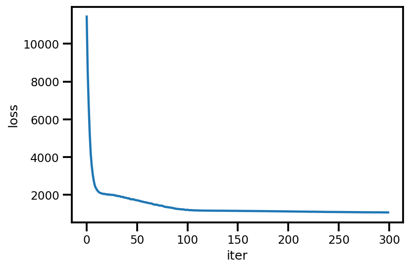
opt = tf.optimizers.Adam(learning_rate=.1)
@tf.function(experimental_compile=True)
def run_approximation():
loss_ = tfp.vi.fit_surrogate_posterior(
contextual_effect_posterior,
surrogate_posterior=advi,
optimizer=opt,
sample_size=10,
num_steps=300)
return loss_
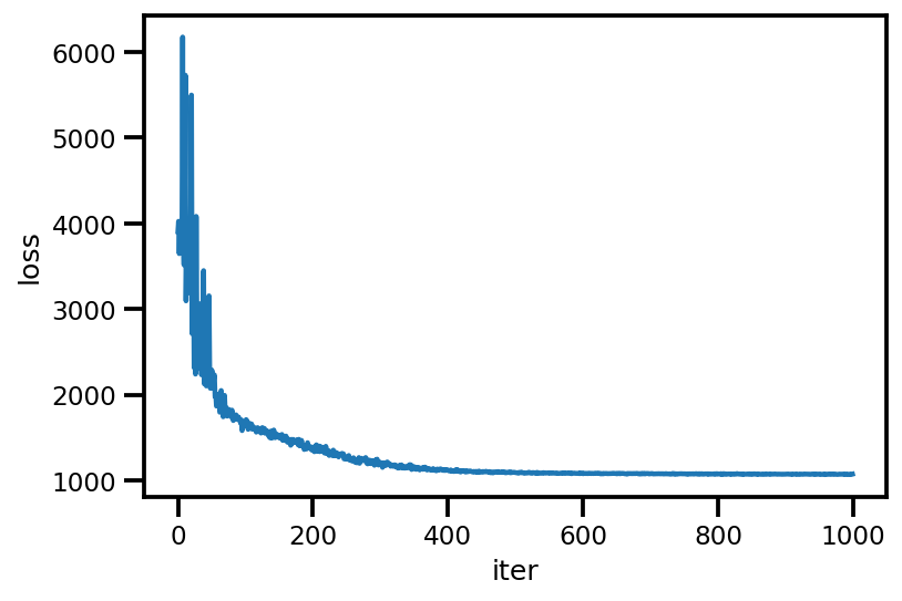
loss_ = run_approximation()
plt.plot(loss_);
plt.xlabel('iter');
plt.ylabel('loss');
graph_info = contextual_effect2.resolve_graph()
approx_param = dict()
free_param = advi.trainable_variables
for i, (rvname, param) in enumerate(graph_info[:-1]):
  approx_param[rvname] = {"mu": free_param[i*2].numpy(),
                          "sd": free_param[i*2+1].numpy()}
approx_param.keys()
dict_keys(['sigma_a', 'eps', 'gamma', 'b', 'sigma_y'])
approx_param['gamma']
{'mu': array([1.28145814, 0.70365287, 1.02689857]),
 'sd': array([-3.6604972 , -2.68153218, -2.04176524])}
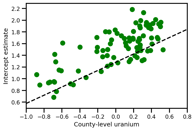
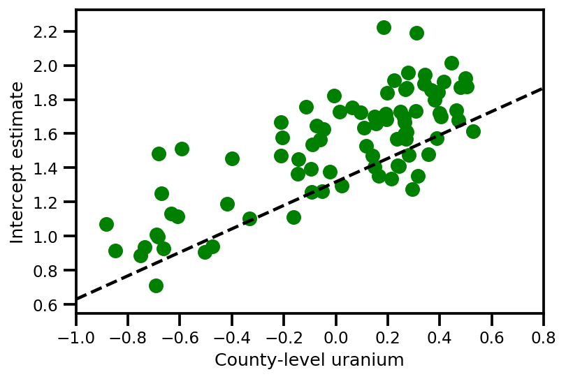
a_means = (approx_param['gamma']['mu'][0]
         + approx_param['gamma']['mu'][1]*u.values
         + approx_param['gamma']['mu'][2]*xbar[county]
         + approx_param['eps']['mu'][county])
_, index = np.unique(county, return_index=True)
plt.scatter(u.values[index], a_means[index], color='g')

xvals = np.linspace(-1, 0.8)
plt.plot(xvals,
         approx_param['gamma']['mu'][0]+approx_param['gamma']['mu'][1]*xvals,
         'k--')
plt.xlim(-1, 0.8)

plt.xlabel('County-level uranium');
plt.ylabel('Intercept estimate');
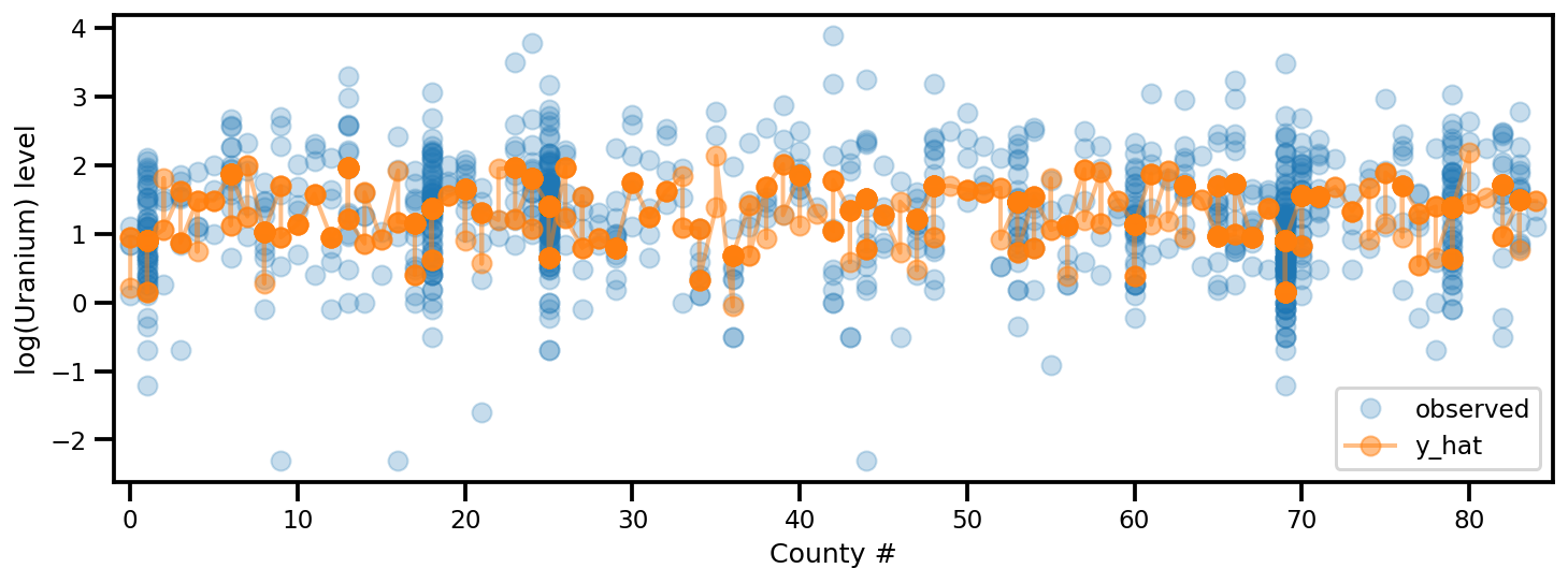
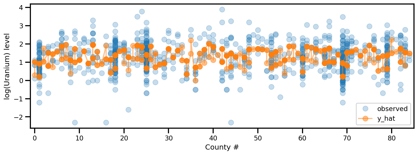
y_est = (approx_param['gamma']['mu'][0]
        + approx_param['gamma']['mu'][1]*u.values
        + approx_param['gamma']['mu'][2]*xbar[county]
        + approx_param['eps']['mu'][county]
        + approx_param['b']['mu']*floor_measure)

_, ax = plt.subplots(1, 1, figsize=(12, 4))
ax.plot(county, log_radon, 'o', alpha=.25, label='observed')
ax.plot(county, y_est, '-o', lw=2, alpha=.5, label='y_hat')
ax.set_xlim(-1, county.max()+1)
plt.legend(loc='lower right')
ax.set_xlabel('County #')
ax.set_ylabel('log(Uranium) level');
Pełna ranga ADVI
W przypadku ADVI pełnej rangi chcemy przybliżyć tył za pomocą wielowymiarowego Gaussa.
USE_FULLRANK = True
*prior_tensors, _ = contextual_effect2.sample()

mapper = Mapper(prior_tensors,
                [tfb.Identity() for _ in prior_tensors],
                contextual_effect2.event_shape[:-1])
rv_shape = ps.shape(mapper.flatten_and_concat(mapper.list_of_tensors))
init_val = tf.random.normal(rv_shape, dtype=dtype)
loc = tf.Variable(init_val, name='loc', dtype=dtype)

if USE_FULLRANK:
  # cov_param = tfp.util.TransformedVariable(
  #     10. * tf.eye(rv_shape[0], dtype=dtype),
  #     tfb.FillScaleTriL(),
  #     name='cov_param'
  #     )
  FillScaleTriL = tfb.FillScaleTriL(
        diag_bijector=tfb.Chain([
          tfb.Shift(tf.cast(.01, dtype)),
          tfb.Softplus(),
          tfb.Shift(tf.cast(np.log(np.expm1(1.)), dtype))]),
        diag_shift=None)
  cov_param = tfp.util.TransformedVariable(
      .02 * tf.eye(rv_shape[0], dtype=dtype),
      FillScaleTriL,
      name='cov_param')
  advi_approx = tfd.MultivariateNormalTriL(
      loc=loc, scale_tril=cov_param)
else:
  # An alternative way to build meanfield ADVI.
  cov_param = tfp.util.TransformedVariable(
      .02 * tf.ones(rv_shape, dtype=dtype),
      tfb.Softplus(),
      name='cov_param'
      )
  advi_approx = tfd.MultivariateNormalDiag(
      loc=loc, scale_diag=cov_param)

contextual_effect_posterior2 = lambda x: contextual_effect_posterior(
    *mapper.split_and_reshape(x)
)

# Check the logp and logq
advi_samples = advi_approx.sample(7)
pprint([
  advi_approx.log_prob(advi_samples),
  contextual_effect_posterior2(advi_samples)
  ])
[<tf.Tensor: shape=(7,), dtype=float64, numpy=
array([238.81841799, 217.71022639, 234.57207103, 230.0643819 ,
       243.73140943, 226.80149702, 232.85184209])>,
 <tf.Tensor: shape=(7,), dtype=float64, numpy=
array([-3638.93663169, -3664.25879314, -3577.69371677, -3696.25705312,
       -3689.12130489, -3777.53698383, -3659.4982734 ])>]
learning_rate = tf.optimizers.schedules.ExponentialDecay(
    initial_learning_rate=1e-2,
    decay_steps=10,
    decay_rate=0.99,
    staircase=True)

opt = tf.optimizers.Adam(learning_rate=learning_rate)

@tf.function(experimental_compile=True)
def run_approximation():
  loss_ = tfp.vi.fit_surrogate_posterior(
        contextual_effect_posterior2,
        surrogate_posterior=advi_approx,
        optimizer=opt,
        sample_size=10,
        num_steps=1000)
  return loss_

loss_ = run_approximation()
plt.plot(loss_);
plt.xlabel('iter');
plt.ylabel('loss');
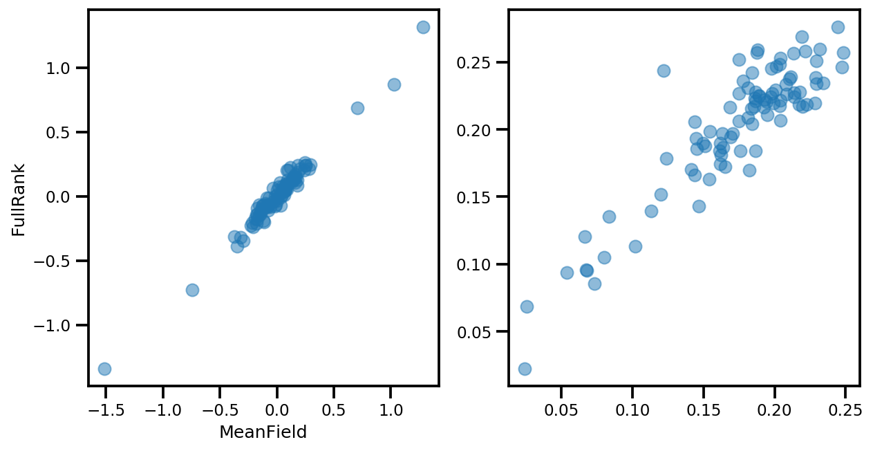
# debug
if True:
  _, ax = plt.subplots(1, 2, figsize=(10, 5))
  ax[0].plot(mapper.flatten_and_concat(advi.mean()), advi_approx.mean(), 'o', alpha=.5)
  ax[1].plot(mapper.flatten_and_concat(advi.stddev()), advi_approx.stddev(), 'o', alpha=.5)
  ax[0].set_xlabel('MeanField')
  ax[0].set_ylabel('FullRank')
graph_info = contextual_effect2.resolve_graph()
approx_param = dict()

free_param_mean = mapper.split_and_reshape(advi_approx.mean())
free_param_std = mapper.split_and_reshape(advi_approx.stddev())
for i, (rvname, param) in enumerate(graph_info[:-1]):
  approx_param[rvname] = {"mu": free_param_mean[i].numpy(),
                          "cov_info": free_param_std[i].numpy()}
a_means = (approx_param['gamma']['mu'][0]
         + approx_param['gamma']['mu'][1]*u.values
         + approx_param['gamma']['mu'][2]*xbar[county]
         + approx_param['eps']['mu'][county])
_, index = np.unique(county, return_index=True)
plt.scatter(u.values[index], a_means[index], color='g')

xvals = np.linspace(-1, 0.8)
plt.plot(xvals,
         approx_param['gamma']['mu'][0]+approx_param['gamma']['mu'][1]*xvals,
         'k--')
plt.xlim(-1, 0.8)

plt.xlabel('County-level uranium');
plt.ylabel('Intercept estimate');
y_est = (approx_param['gamma']['mu'][0]
         + approx_param['gamma']['mu'][1]*u.values
         + approx_param['gamma']['mu'][2]*xbar[county]
         + approx_param['eps']['mu'][county]
         + approx_param['b']['mu']*floor_measure)

_, ax = plt.subplots(1, 1, figsize=(12, 4))
ax.plot(county, log_radon, 'o', alpha=.25, label='observed')
ax.plot(county, y_est, '-o', lw=2, alpha=.5, label='y_hat')
ax.set_xlim(-1, county.max()+1)
plt.legend(loc='lower right')
ax.set_xlabel('County #')
ax.set_ylabel('log(Uranium) level');
Model mieszaniny Beta-Bernoulliego
Model mieszaniny, w którym wielu recenzentów etykietuje niektóre elementy z nieznanymi (prawdziwymi) ukrytymi etykietami.
dtype = tf.float32
n = 50000    # number of examples reviewed
p_bad_ = 0.1 # fraction of bad events
m = 5        # number of reviewers for each example
rcl_ = .35 + np.random.rand(m)/10
prc_ = .65 + np.random.rand(m)/10

# PARAMETER TRANSFORMATION
tpr = rcl_
fpr = p_bad_*tpr*(1./prc_-1.)/(1.-p_bad_)
tnr = 1 - fpr

# broadcast to m reviewer.
batch_prob = np.asarray([tpr, fpr]).T
mixture = tfd.Mixture(
    tfd.Categorical(
        probs=[p_bad_, 1-p_bad_]),
    [
        tfd.Independent(tfd.Bernoulli(probs=tpr), 1),
        tfd.Independent(tfd.Bernoulli(probs=fpr), 1),
    ])
# Generate reviewer response
X_tf = mixture.sample([n])

# run once to always use the same array as input
# so we can compare the estimation from different
# inference method.
X_np = X_tf.numpy()
# batched Mixture model
mdl_mixture = tfd.JointDistributionSequential([
    tfd.Sample(tfd.Beta(5., 2.), m),
    tfd.Sample(tfd.Beta(2., 2.), m),
    tfd.Sample(tfd.Beta(1., 10), 1),
    lambda p_bad, rcl, prc: tfd.Sample(
        tfd.Mixture(
            tfd.Categorical(
                probs=tf.concat([p_bad, 1.-p_bad], -1)),
            [
              tfd.Independent(tfd.Bernoulli(
                  probs=rcl), 1),
              tfd.Independent(tfd.Bernoulli(
                  probs=p_bad*rcl*(1./prc-1.)/(1.-p_bad)), 1)
             ]
      ), (n, )),
    ])

mdl_mixture.resolve_graph()
(('prc', ()), ('rcl', ()), ('p_bad', ()), ('x', ('p_bad', 'rcl', 'prc')))
prc, rcl, p_bad, x = mdl_mixture.sample(4)
x.shape
TensorShape([4, 50000, 5])
mdl_mixture.log_prob_parts([prc, rcl, p_bad, X_np[np.newaxis, ...]])
[<tf.Tensor: shape=(4,), dtype=float32, numpy=array([1.4828572, 2.957961 , 2.9355168, 2.6116824], dtype=float32)>,
 <tf.Tensor: shape=(4,), dtype=float32, numpy=array([-0.14646745,  1.3308513 ,  1.1205603 ,  0.5441705 ], dtype=float32)>,
 <tf.Tensor: shape=(4,), dtype=float32, numpy=array([1.3733709, 1.8020535, 2.1865845, 1.5701319], dtype=float32)>,
 <tf.Tensor: shape=(4,), dtype=float32, numpy=array([-54326.664, -52683.93 , -64407.67 , -55007.895], dtype=float32)>]
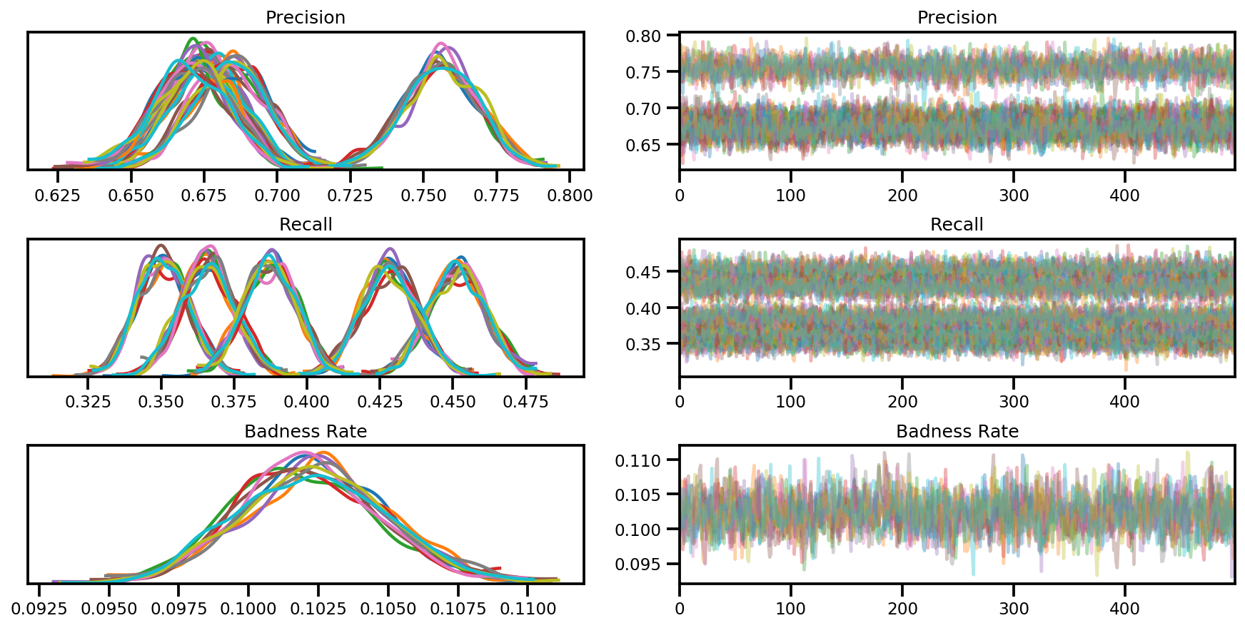
Wnioskowanie (NUTS)
nchain = 10
prc, rcl, p_bad, _ = mdl_mixture.sample(nchain)
initial_chain_state = [prc, rcl, p_bad]

# Since MCMC operates over unconstrained space, we need to transform the
# samples so they live in real-space.
unconstraining_bijectors = [
    tfb.Sigmoid(),       # Maps R to [0, 1].
    tfb.Sigmoid(),       # Maps R to [0, 1].
    tfb.Sigmoid(),       # Maps R to [0, 1].
]
step_size = [tf.cast(i, dtype=dtype) for i in [1e-3, 1e-3, 1e-3]]

X_expanded = X_np[np.newaxis, ...]
target_log_prob_fn = lambda *x: mdl_mixture.log_prob(x + (X_expanded, ))

samples, sampler_stat = run_chain(
    initial_chain_state, step_size, target_log_prob_fn,
    unconstraining_bijectors, burnin=100)
# using the pymc3 naming convention
sample_stats_name = ['lp', 'tree_size', 'diverging', 'energy', 'mean_tree_accept']
sample_stats = {k:v.numpy().T for k, v in zip(sample_stats_name, sampler_stat)}
sample_stats['tree_size'] = np.diff(sample_stats['tree_size'], axis=1)

var_name = ['Precision', 'Recall', 'Badness Rate']
posterior = {k:np.swapaxes(v.numpy(), 1, 0)
             for k, v in zip(var_name, samples)}

az_trace = az.from_dict(posterior=posterior, sample_stats=sample_stats)
axes = az.plot_trace(az_trace, compact=True);