| | |  Wyświetl źródło na GitHub Wyświetl źródło na GitHub | |
To jest port prawdopodobieństwa TensorFlow z tytułowego artykułu Li i in. z 16 marca 2020 r. Wiernie odtwarzamy metody i wyniki oryginalnych autorów na platformie TensorFlow Probability, prezentując niektóre możliwości TFP w kontekście nowoczesnego modelowania epidemiologicznego. Przeniesienie do TensorFlow zapewnia nam ~10-krotne przyspieszenie w stosunku do oryginalnego kodu Matlab, a ponieważ TensorFlow Probability wszechstronnie obsługuje wektoryzowane obliczenia wsadowe, również korzystnie skaluje się do setek niezależnych replikacji.
Oryginalny papier
Ruiyun Li, Sen Pei, Bin Chen, Yimeng Song, Tao Zhang, Wan Yang i Jeffrey Shaman. Poważna nieudokumentowana infekcja ułatwia szybkie rozprzestrzenianie się nowego koronawirusa (SARS-CoV2). (2020), doi: https://doi.org/10.1126/science.abb3221 .
Streszczenie:. „Ocena częstości występowania i zaraźliwość z nielegalnych powieść koronawirus (SARS-CoV2) Zakażenia ma kluczowe znaczenie dla zrozumienia ogólnej chorobowości i pandemii potencjał tej choroby Tutaj używamy uwag zgłoszonych zakażeń w Chinach, w połączeniu z danymi z mobilnością, a sieciowy model dynamicznej metapopulacji i wnioskowanie bayesowskie w celu wywnioskowania krytycznych cech epidemiologicznych związanych z SARS-CoV2, w tym frakcji nieudokumentowanych infekcji i ich zaraźliwości Szacujemy, że 86% wszystkich infekcji było nieudokumentowanych (95% CI: [82%–90%]). ) przed ograniczeniami w podróżowaniu do 23 stycznia 2020 r. Na osobę wskaźnik przenoszenia nieudokumentowanych infekcji wyniósł 55% udokumentowanych infekcji ([46%–62%]), jednak ze względu na ich większą liczbę, nieudokumentowane infekcje były źródłem infekcji dla 79 % udokumentowanych przypadków. Te odkrycia wyjaśniają szybkie geograficzne rozprzestrzenianie się SARS-CoV2 i wskazują, że powstrzymanie tego wirusa będzie szczególnie trudne”.
Github odwołuje się do kodu i danych.
Przegląd
Model jest przedziałowego modelu choroby , z przegrodami dla „podatny”, „odsłonięta” (zakażonych, ale jeszcze nie zakaźna) „nie udokumentowane zakażenie” lub „ewentualnie udokumentowane zakaźna”. Na uwagę zasługują dwie cechy: oddzielne przedziały dla każdego z 375 chińskich miast, z założeniem o tym, jak ludzie podróżują z jednego miasta do drugiego; i opóźnienia w sprawozdawczości infekcji, tak, że to przypadek, że staje się „ostatecznie udokumentowane zakaźny” na dzień \(t\) nie pokazać się w zaobserwowanych przypadków liczy aż stochastycznego późniejszym dniu.
Model zakłada, że przypadki nigdy nieudokumentowane są nieudokumentowane jako łagodniejsze, a tym samym zarażają innych w mniejszym stopniu. Głównym parametrem będącym przedmiotem zainteresowania w oryginalnej pracy jest odsetek przypadków, które pozostają nieudokumentowane, aby oszacować zarówno zasięg istniejącej infekcji, jak i wpływ nieudokumentowanej transmisji na rozprzestrzenianie się choroby.
Ta współpraca ma strukturę przewodnika po kodzie w stylu oddolnym. W porządku, będziemy
- Przyjmuj i krótko analizuj dane,
- Zdefiniuj przestrzeń stanów i dynamikę modelu,
- Zbuduj zestaw funkcji do wnioskowania w modelu zgodnie z Li i in., oraz
- Przywołaj je i zbadaj wyniki. Spoiler: Wychodzą tak samo jak papier.
Instalacja i importy Pythona
pip3 install -q tf-nightly tfp-nightly
import collections
import io
import requests
import time
import zipfile

import matplotlib.pyplot as plt
import numpy as np
import pandas as pd

import tensorflow.compat.v2 as tf
import tensorflow_probability as tfp
from tensorflow_probability.python.internal import samplers

tfd = tfp.distributions
tfes = tfp.experimental.sequential
Import danych
Zaimportujmy dane z github i sprawdźmy niektóre z nich.
r = requests.get('https://raw.githubusercontent.com/SenPei-CU/COVID-19/master/Data.zip')
z = zipfile.ZipFile(io.BytesIO(r.content))
z.extractall('/tmp/')
raw_incidence = pd.read_csv('/tmp/data/Incidence.csv')
raw_mobility = pd.read_csv('/tmp/data/Mobility.csv')
raw_population = pd.read_csv('/tmp/data/pop.csv')
Poniżej możemy zobaczyć surową liczbę zachorowań na dzień. Najbardziej interesują nas pierwsze 14 dni (od 10 stycznia do 23 stycznia), ponieważ 23 stycznia wprowadzono ograniczenia w podróżowaniu. Artykuł zajmuje się tym poprzez oddzielne modelowanie 10–23 stycznia i 23 stycznia + z różnymi parametrami; ograniczymy się tylko do okresu rozmnażania się we wcześniejszym okresie.
raw_incidence.drop('Date', axis=1)  # The 'Date' column is all 1/18/21
# Luckily the days are in order, starting on January 10th, 2020.
Sprawdźmy, ile zachorowań przypada na Wuhan.
plt.plot(raw_incidence.Wuhan, '.-')
plt.title('Wuhan incidence counts over 1/10/20 - 02/08/20')
plt.show()
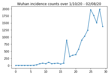
Jak na razie dobrze. Teraz liczy się populacja początkowa.
raw_population
Sprawdźmy też i zapiszmy, który wpis to Wuhan.
raw_population['City'][169]
'Wuhan'
WUHAN_IDX = 169
I tutaj widzimy macierz mobilności między różnymi miastami. Jest to przybliżona liczba osób przemieszczających się między różnymi miastami w ciągu pierwszych 14 dni. Pochodzi z zapisów GPS dostarczonych przez Tencent na sezon 2018 Księżycowego Nowego Roku. Li i wsp ruchliwość modelu podczas sezonu 2020 jako jakiś nieznany (w zależności od wnioskowanie) stały współczynnik \(\theta\) czasie to.
raw_mobility
Na koniec przetwórzmy to wszystko w numpy tablice, które możemy wykorzystać.
# The given populations are only "initial" because of intercity mobility during
# the holiday season.
initial_population = raw_population['Population'].to_numpy().astype(np.float32)
Przekształć dane mobilności w tensor w kształcie [L, L, T], gdzie L to liczba lokalizacji, a T to liczba kroków czasowych.
daily_mobility_matrices = []
for i in range(1, 15):
  day_mobility = raw_mobility[raw_mobility['Day'] == i]

  # Make a matrix of daily mobilities.
  z = pd.crosstab(
      day_mobility.Origin,
      day_mobility.Destination,
      values=day_mobility['Mobility Index'], aggfunc='sum', dropna=False)

  # Include every city, even if there are no rows for some in the raw data on
  # some day.  This uses the sort order of `raw_population`.
  z = z.reindex(index=raw_population['City'], columns=raw_population['City'],
                fill_value=0)
  # Finally, fill any missing entries with 0. This means no mobility.
  z = z.fillna(0)
  daily_mobility_matrices.append(z.to_numpy())

mobility_matrix_over_time = np.stack(daily_mobility_matrices, axis=-1).astype(
    np.float32)
Na koniec weź zaobserwowane infekcje i sporządź tabelę [L, T].
# Remove the date parameter and take the first 14 days.
observed_daily_infectious_count = raw_incidence.to_numpy()[:14, 1:]
observed_daily_infectious_count = np.transpose(
    observed_daily_infectious_count).astype(np.float32)
I jeszcze raz sprawdź, czy otrzymaliśmy kształty tak, jak chcieliśmy. Przypominamy, że współpracujemy z 375 miastami i 14 dniami.
print('Mobility Matrix over time should have shape (375, 375, 14): {}'.format(
    mobility_matrix_over_time.shape))
print('Observed Infectious should have shape (375, 14): {}'.format(
    observed_daily_infectious_count.shape))
print('Initial population should have shape (375): {}'.format(
    initial_population.shape))
Mobility Matrix over time should have shape (375, 375, 14): (375, 375, 14)
Observed Infectious should have shape (375, 14): (375, 14)
Initial population should have shape (375): (375,)
Definiowanie stanu i parametrów
Zacznijmy definiować nasz model. Model jesteśmy reprodukcji jest wariantem modelu Seir . W tym przypadku mamy do czynienia z następującymi stanami zmiennymi w czasie:
- \(S\): Liczba osób podatnych na choroby w każdym mieście.
- \(E\): Liczba osób w każdym mieście narażonych na choroby zakaźne, ale nie jeszcze. Z biologicznego punktu widzenia odpowiada to zarażeniu chorobą, ponieważ wszyscy narażeni ludzie w końcu stają się zaraźliwi.
- \(I^u\): Liczba osób w każdym mieście, którzy są zakaźne, ale nieudokumentowane. W modelu oznacza to właściwie „nigdy nie zostanie udokumentowane”.
- \(I^r\): Liczba osób w każdym mieście, którzy są zakaźne i udokumentowane jako takie. Li i wsp modelowe opóźnienia raportowania, więc \(I^r\) faktycznie odpowiada coś takiego jak „sprawy jest wystarczająco ciężkie powinny być udokumentowane w pewnym momencie w przyszłości”.
Jak zobaczymy poniżej, będziemy wnioskować o tych stanach, uruchamiając filtr Kalmana dostosowany do zestawu (EAKF) do przodu w czasie. Wektor stanu EAKF to jeden wektor z indeksem miasta dla każdej z tych wielkości.
Model ma następujące możliwe do wywnioskowania globalne, niezmienne w czasie parametry:
- \(\beta\): Szybkość transmisji ze względu na udokumentowane zakaźnych jednostek.
- \(\mu\): Względna szybkość transmisji ze względu na osoby nieudokumentowanych-zakaźny. Będzie to działać przez produkt \(\mu \beta\).
- \(\theta\): Współczynnik mobilności intercity. Jest to czynnik większy niż 1, korygujący niedoszacowanie danych dotyczących mobilności (i wzrostu populacji w latach 2018-2020).
- \(Z\): Średni okres inkubacji (czyli czas, w „narażonych” państwa).
- \(\alpha\): Jest to frakcja zakażeń na tyle silne, aby być (ewentualnie) udokumentowane.
- \(D\): Średni czas trwania infekcji (czyli czas w obu „zakaźne” państwa).
Będziemy wnioskować oszacowania punktowe dla tych parametrów za pomocą pętli iteracyjnego filtrowania wokół EAKF dla stanów.
Model zależy również od stałych niewnioskowanych:
- \(M\): Matryca ruchliwość lokalne. Jest to zmienne w czasie i przypuszczalnie dane. Przypomnijmy, że to skalowane przez wywnioskować parametru \(\theta\) dać rzeczywiste ruchy ludności między miastami.
- \(N\): Łączna liczba osób w każdym mieście. Początkowe populacje są pobierane dane, a czasem zmiana populacji jest obliczana na podstawie liczby mobilności \(\theta M\).
Najpierw dajemy sobie pewne struktury danych do przechowywania naszych stanów i parametrów.
SEIRComponents = collections.namedtuple(
  typename='SEIRComponents',
  field_names=[
    'susceptible',              # S
    'exposed',                  # E
    'documented_infectious',    # I^r
    'undocumented_infectious',  # I^u
    # This is the count of new cases in the "documented infectious" compartment.
    # We need this because we will introduce a reporting delay, between a person
    # entering I^r and showing up in the observable case count data.
    # This can't be computed from the cumulative `documented_infectious` count,
    # because some portion of that population will move to the 'recovered'
    # state, which we aren't tracking explicitly.
    'daily_new_documented_infectious'])

ModelParams = collections.namedtuple(
    typename='ModelParams',
    field_names=[
      'documented_infectious_tx_rate',             # Beta
      'undocumented_infectious_tx_relative_rate',  # Mu
      'intercity_underreporting_factor',           # Theta
      'average_latency_period',                    # Z
      'fraction_of_documented_infections',         # Alpha
      'average_infection_duration'                 # D
    ]
)
Kodujemy również granice Li i innych dla wartości parametrów.
PARAMETER_LOWER_BOUNDS = ModelParams(
    documented_infectious_tx_rate=0.8,
    undocumented_infectious_tx_relative_rate=0.2,
    intercity_underreporting_factor=1.,
    average_latency_period=2.,
    fraction_of_documented_infections=0.02,
    average_infection_duration=2.
)

PARAMETER_UPPER_BOUNDS = ModelParams(
    documented_infectious_tx_rate=1.5,
    undocumented_infectious_tx_relative_rate=1.,
    intercity_underreporting_factor=1.75,
    average_latency_period=5.,
    fraction_of_documented_infections=1.,
    average_infection_duration=5.
)
SEIR Dynamika
Tutaj definiujemy relację między parametrami a stanem.
Równania dynamiki w czasie z Li i in. (materiał uzupełniający, eqns 1-5) są następujące:
\(\frac{dS_i}{dt} = -\beta \frac{S_i I_i^r}{N_i} - \mu \beta \frac{S_i I_i^u}{N_i} + \theta \sum_k \frac{M_{ij} S_j}{N_j - I_j^r} - + \theta \sum_k \frac{M_{ji} S_j}{N_i - I_i^r}\)
\(\frac{dE_i}{dt} = \beta \frac{S_i I_i^r}{N_i} + \mu \beta \frac{S_i I_i^u}{N_i} -\frac{E_i}{Z} + \theta \sum_k \frac{M_{ij} E_j}{N_j - I_j^r} - + \theta \sum_k \frac{M_{ji} E_j}{N_i - I_i^r}\)
\(\frac{dI^r_i}{dt} = \alpha \frac{E_i}{Z} - \frac{I_i^r}{D}\)
\(\frac{dI^u_i}{dt} = (1 - \alpha) \frac{E_i}{Z} - \frac{I_i^u}{D} + \theta \sum_k \frac{M_{ij} I_j^u}{N_j - I_j^r} - + \theta \sum_k \frac{M_{ji} I^u_j}{N_i - I_i^r}\)
\(N_i = N_i + \theta \sum_j M_{ij} - \theta \sum_j M_{ji}\)
Dla przypomnienia, w \(i\) i \(j\) miastach indeksy dolne. Te równania modelują ewolucję choroby w czasie przez
- Kontakt z osobami zakaźnymi prowadzący do większej infekcji;
- Progresja choroby od „narażonej” do jednego ze stanów „zakaźnych”;
- Progresja choroby od stanu „zakaźnego” do wyzdrowienia, którą modelujemy przez usunięcie z modelowanej populacji;
- Mobilność międzymiastowa, w tym osoby narażone lub nieudokumentowane zakażone; oraz
- Zmienność czasowa populacji miast w ciągu dnia poprzez mobilność między miastami.
Za Li i wsp. zakładamy, że osoby, u których przypadki są na tyle poważne, że w końcu zostaną zgłoszone, nie podróżują między miastami.
Również podążając za Li et al, traktujemy tę dynamikę jako podlegającą szumowi Poissona w zakresie terminów, tj. każdy termin jest w rzeczywistości współczynnikiem Poissona, z którego próbka daje prawdziwą zmianę. Szum Poissona jest terminowy, ponieważ odejmowanie (w przeciwieństwie do dodawania) próbek Poissona nie daje wyniku z rozkładem Poissona.
Będziemy rozwijać tę dynamikę w czasie za pomocą klasycznego integratora czwartego rzędu Runge-Kutta, ale najpierw zdefiniujmy funkcję, która je oblicza (w tym próbkowanie szumu Poissona).
def sample_state_deltas(
    state, population, mobility_matrix, params, seed, is_deterministic=False):
  """Computes one-step change in state, including Poisson sampling.

  Note that this is coded to support vectorized evaluation on arbitrary-shape
  batches of states.  This is useful, for example, for running multiple
  independent replicas of this model to compute credible intervals for the
  parameters.  We refer to the arbitrary batch shape with the conventional
  `B` in the parameter documentation below.  This function also, of course,
  supports broadcasting over the batch shape.

  Args:
    state: A `SEIRComponents` tuple with fields Tensors of shape
      B + [num_locations] giving the current disease state.
    population: A Tensor of shape B + [num_locations] giving the current city
      populations.
    mobility_matrix: A Tensor of shape B + [num_locations, num_locations] giving
      the current baseline inter-city mobility.
    params: A `ModelParams` tuple with fields Tensors of shape B giving the
      global parameters for the current EAKF run.
    seed: Initial entropy for pseudo-random number generation.  The Poisson
      sampling is repeatable by supplying the same seed.
    is_deterministic: A `bool` flag to turn off Poisson sampling if desired.

  Returns:
    delta: A `SEIRComponents` tuple with fields Tensors of shape
      B + [num_locations] giving the one-day changes in the state, according
      to equations 1-4 above (including Poisson noise per Li et al).
  """
  undocumented_infectious_fraction = state.undocumented_infectious / population
  documented_infectious_fraction = state.documented_infectious / population

  # Anyone not documented as infectious is considered mobile
  mobile_population = (population - state.documented_infectious)
  def compute_outflow(compartment_population):
    raw_mobility = tf.linalg.matvec(
        mobility_matrix, compartment_population / mobile_population)
    return params.intercity_underreporting_factor * raw_mobility
  def compute_inflow(compartment_population):
    raw_mobility = tf.linalg.matmul(
        mobility_matrix,
        (compartment_population / mobile_population)[..., tf.newaxis],
        transpose_a=True)
    return params.intercity_underreporting_factor * tf.squeeze(
        raw_mobility, axis=-1)

  # Helper for sampling the Poisson-variate terms.
  seeds = samplers.split_seed(seed, n=11)
  if is_deterministic:
    def sample_poisson(rate):
      return rate
  else:
    def sample_poisson(rate):
      return tfd.Poisson(rate=rate).sample(seed=seeds.pop())

  # Below are the various terms called U1-U12 in the paper. We combined the
  # first two, which should be fine; both are poisson so their sum is too, and
  # there's no risk (as there could be in other terms) of going negative.
  susceptible_becoming_exposed = sample_poisson(
      state.susceptible *
      (params.documented_infectious_tx_rate *
       documented_infectious_fraction +
       (params.undocumented_infectious_tx_relative_rate *
        params.documented_infectious_tx_rate) *
       undocumented_infectious_fraction))  # U1 + U2

  susceptible_population_inflow = sample_poisson(
      compute_inflow(state.susceptible))  # U3
  susceptible_population_outflow = sample_poisson(
      compute_outflow(state.susceptible))  # U4

  exposed_becoming_documented_infectious = sample_poisson(
      params.fraction_of_documented_infections *
      state.exposed / params.average_latency_period)  # U5
  exposed_becoming_undocumented_infectious = sample_poisson(
      (1 - params.fraction_of_documented_infections) *
      state.exposed / params.average_latency_period)  # U6

  exposed_population_inflow = sample_poisson(
      compute_inflow(state.exposed))  # U7
  exposed_population_outflow = sample_poisson(
      compute_outflow(state.exposed))  # U8

  documented_infectious_becoming_recovered = sample_poisson(
      state.documented_infectious /
      params.average_infection_duration)  # U9
  undocumented_infectious_becoming_recovered = sample_poisson(
      state.undocumented_infectious /
      params.average_infection_duration)  # U10

  undocumented_infectious_population_inflow = sample_poisson(
      compute_inflow(state.undocumented_infectious))  # U11
  undocumented_infectious_population_outflow = sample_poisson(
      compute_outflow(state.undocumented_infectious))  # U12

  # The final state_deltas
  return SEIRComponents(
      # Equation [1]
      susceptible=(-susceptible_becoming_exposed +
                   susceptible_population_inflow +
                   -susceptible_population_outflow),
      # Equation [2]
      exposed=(susceptible_becoming_exposed +
               -exposed_becoming_documented_infectious +
               -exposed_becoming_undocumented_infectious +
               exposed_population_inflow +
               -exposed_population_outflow),
      # Equation [3]
      documented_infectious=(
          exposed_becoming_documented_infectious +
          -documented_infectious_becoming_recovered),
      # Equation [4]
      undocumented_infectious=(
          exposed_becoming_undocumented_infectious +
          -undocumented_infectious_becoming_recovered +
          undocumented_infectious_population_inflow +
          -undocumented_infectious_population_outflow),
      # New to-be-documented infectious cases, subject to the delayed
      # observation model.
      daily_new_documented_infectious=exposed_becoming_documented_infectious)
Oto integrator. To jest całkowicie standard, z wyjątkiem nasion PRNG przechodzącej przez do sample_state_deltas funkcjonować, aby uzyskać niezależne szum Poissona na siebie częściowych kroków, jakie Runge-Kutty połączeń metoda.
@tf.function(autograph=False)
def rk4_one_step(state, population, mobility_matrix, params, seed):
  """Implement one step of RK4, wrapped around a call to sample_state_deltas."""
  # One seed for each RK sub-step
  seeds = samplers.split_seed(seed, n=4)

  deltas = tf.nest.map_structure(tf.zeros_like, state)
  combined_deltas = tf.nest.map_structure(tf.zeros_like, state)

  for a, b in zip([1., 2, 2, 1.], [6., 3., 3., 6.]):
    next_input = tf.nest.map_structure(
        lambda x, delta, a=a: x + delta / a, state, deltas)
    deltas = sample_state_deltas(
        next_input,
        population,
        mobility_matrix,
        params,
        seed=seeds.pop(), is_deterministic=False)
    combined_deltas = tf.nest.map_structure(
        lambda x, delta, b=b: x + delta / b, combined_deltas, deltas)

  return tf.nest.map_structure(
      lambda s, delta: s + tf.round(delta),
      state, combined_deltas)
Inicjalizacja
Tutaj wdrażamy schemat inicjalizacji z papieru.
Zgodnie z Li i in., naszym schematem wnioskowania będzie wewnętrzna pętla filtru Kalmana dopasowująca zespół, otoczona iterowaną zewnętrzną pętlą filtrowania (IF-EAKF). Obliczeniowo oznacza to, że potrzebujemy trzech rodzajów inicjalizacji:
- Stan początkowy dla wewnętrznego EAKF
- Parametry początkowe dla zewnętrznego IF, które są jednocześnie parametrami początkowymi dla pierwszego EAKF
- Aktualizowanie parametrów z jednej iteracji IF do następnej, które służą jako parametry początkowe dla każdego EAKF innego niż pierwszy.
def initialize_state(num_particles, num_batches, seed):
  """Initialize the state for a batch of EAKF runs.

  Args:
    num_particles: `int` giving the number of particles for the EAKF.
    num_batches: `int` giving the number of independent EAKF runs to
      initialize in a vectorized batch.
    seed: PRNG entropy.

  Returns:
    state: A `SEIRComponents` tuple with Tensors of shape [num_particles,
      num_batches, num_cities] giving the initial conditions in each
      city, in each filter particle, in each batch member.
  """
  num_cities = mobility_matrix_over_time.shape[-2]
  state_shape = [num_particles, num_batches, num_cities]
  susceptible = initial_population * np.ones(state_shape, dtype=np.float32)
  documented_infectious = np.zeros(state_shape, dtype=np.float32)
  daily_new_documented_infectious = np.zeros(state_shape, dtype=np.float32)

  # Following Li et al, initialize Wuhan with up to 2000 people exposed
  # and another up to 2000 undocumented infectious.
  rng = np.random.RandomState(seed[0] % (2**31 - 1))
  wuhan_exposed = rng.randint(
      0, 2001, [num_particles, num_batches]).astype(np.float32)
  wuhan_undocumented_infectious = rng.randint(
      0, 2001, [num_particles, num_batches]).astype(np.float32)

  # Also following Li et al, initialize cities adjacent to Wuhan with three
  # days' worth of additional exposed and undocumented-infectious cases,
  # as they may have traveled there before the beginning of the modeling
  # period.
  exposed = 3 * mobility_matrix_over_time[
      WUHAN_IDX, :, 0] * wuhan_exposed[
          ..., np.newaxis] / initial_population[WUHAN_IDX]
  undocumented_infectious = 3 * mobility_matrix_over_time[
      WUHAN_IDX, :, 0] * wuhan_undocumented_infectious[
          ..., np.newaxis] / initial_population[WUHAN_IDX]

  exposed[..., WUHAN_IDX] = wuhan_exposed
  undocumented_infectious[..., WUHAN_IDX] = wuhan_undocumented_infectious

  # Following Li et al, we do not remove the inital exposed and infectious
  # persons from the susceptible population.
  return SEIRComponents(
      susceptible=tf.constant(susceptible),
      exposed=tf.constant(exposed),
      documented_infectious=tf.constant(documented_infectious),
      undocumented_infectious=tf.constant(undocumented_infectious),
      daily_new_documented_infectious=tf.constant(daily_new_documented_infectious))

def initialize_params(num_particles, num_batches, seed):
  """Initialize the global parameters for the entire inference run.

  Args:
    num_particles: `int` giving the number of particles for the EAKF.
    num_batches: `int` giving the number of independent EAKF runs to
      initialize in a vectorized batch.
    seed: PRNG entropy.

  Returns:
    params: A `ModelParams` tuple with fields Tensors of shape
      [num_particles, num_batches] giving the global parameters
      to use for the first batch of EAKF runs.
  """
  # We have 6 parameters. We'll initialize with a Sobol sequence,
  # covering the hyper-rectangle defined by our parameter limits.
  halton_sequence = tfp.mcmc.sample_halton_sequence(
      dim=6, num_results=num_particles * num_batches, seed=seed)
  halton_sequence = tf.reshape(
      halton_sequence, [num_particles, num_batches, 6])
  halton_sequences = tf.nest.pack_sequence_as(
      PARAMETER_LOWER_BOUNDS, tf.split(
          halton_sequence, num_or_size_splits=6, axis=-1))
  def interpolate(minval, maxval, h):
    return (maxval - minval) * h + minval
  return tf.nest.map_structure(
      interpolate,
      PARAMETER_LOWER_BOUNDS, PARAMETER_UPPER_BOUNDS, halton_sequences)

def update_params(num_particles, num_batches,
                  prev_params, parameter_variance, seed):
  """Update the global parameters between EAKF runs.

  Args:
    num_particles: `int` giving the number of particles for the EAKF.
    num_batches: `int` giving the number of independent EAKF runs to
      initialize in a vectorized batch.
    prev_params: A `ModelParams` tuple of the parameters used for the previous
      EAKF run.
    parameter_variance: A `ModelParams` tuple specifying how much to drift
      each parameter.
    seed: PRNG entropy.

  Returns:
    params: A `ModelParams` tuple with fields Tensors of shape
      [num_particles, num_batches] giving the global parameters
      to use for the next batch of EAKF runs.
  """
  # Initialize near the previous set of parameters. This is the first step
  # in Iterated Filtering.
  seeds = tf.nest.pack_sequence_as(
      prev_params, samplers.split_seed(seed, n=len(prev_params)))
  return tf.nest.map_structure(
      lambda x, v, seed: x + tf.math.sqrt(v) * tf.random.stateless_normal([
          num_particles, num_batches, 1], seed=seed),
      prev_params, parameter_variance, seeds)
Opóźnienia
Jedną z ważnych cech tego modelu jest wyraźne uwzględnienie faktu, że infekcje są zgłaszane później niż się zaczynają. Oznacza to, że możemy spodziewać się, że osoba, która porusza się z \(E\) komory do \(I^r\) komory na dzień \(t\) nie może pokazać się w obserwowalnych zgłoszony przypadek liczy aż późniejszym dniu.
Zakładamy, że opóźnienie ma rozkład gamma. Zgodnie z Li i in. używamy 1,85 dla kształtu i sparametryzujemy szybkość, aby uzyskać średnie opóźnienie raportowania wynoszące 9 dni.
def raw_reporting_delay_distribution(gamma_shape=1.85, reporting_delay=9.):
  return tfp.distributions.Gamma(
      concentration=gamma_shape, rate=gamma_shape / reporting_delay)
Nasze obserwacje są dyskretne, więc surowe (ciągłe) opóźnienia będziemy zaokrąglać do najbliższego dnia. Mamy też skończony horyzont danych, więc rozkład opóźnień dla jednej osoby jest kategoryczny w pozostałych dniach. Możemy więc obliczyć za-miasto przewidywane obserwacje bardziej efektywnie niż próbkowanie \(O(I^r)\) gamma, przez pre-computing wielomianowych prawdopodobieństw opóźnienia zamiast.
def reporting_delay_probs(num_timesteps, gamma_shape=1.85, reporting_delay=9.):
  gamma_dist = raw_reporting_delay_distribution(gamma_shape, reporting_delay)
  multinomial_probs = [gamma_dist.cdf(1.)]
  for k in range(2, num_timesteps + 1):
    multinomial_probs.append(gamma_dist.cdf(k) - gamma_dist.cdf(k - 1))
  # For samples that are larger than T.
  multinomial_probs.append(gamma_dist.survival_function(num_timesteps))
  multinomial_probs = tf.stack(multinomial_probs)
  return multinomial_probs
Oto kod do faktycznego zastosowania tych opóźnień do nowych, udokumentowanych codziennie liczby infekcji:
def delay_reporting(
    daily_new_documented_infectious, num_timesteps, t, multinomial_probs, seed):
  # This is the distribution of observed infectious counts from the current
  # timestep.

  raw_delays = tfd.Multinomial(
      total_count=daily_new_documented_infectious,
      probs=multinomial_probs).sample(seed=seed)

  # The last bucket is used for samples that are out of range of T + 1. Thus
  # they are not going to be observable in this model.
  clipped_delays = raw_delays[..., :-1]

  # We can also remove counts that are such that t + i >= T.
  clipped_delays = clipped_delays[..., :num_timesteps - t]
  # We finally shift everything by t. That means prepending with zeros.
  return tf.concat([
      tf.zeros(
          tf.concat([
              tf.shape(clipped_delays)[:-1], [t]], axis=0),
          dtype=clipped_delays.dtype),
      clipped_delays], axis=-1)
Wnioskowanie
Najpierw zdefiniujemy niektóre struktury danych do wnioskowania.
W szczególności będziemy chcieli przeprowadzić filtrowanie iteracyjne, które pakuje stan i parametry razem podczas wnioskowania. Będziemy więc zdefiniować ParameterStatePair obiekt.
Chcemy również dołączyć do modelu wszelkie informacje poboczne.
ParameterStatePair = collections.namedtuple(
    'ParameterStatePair', ['state', 'params'])

# Info that is tracked and mutated but should not have inference performed over.
SideInfo = collections.namedtuple(
    'SideInfo', [
        # Observations at every time step.
        'observations_over_time',
        'initial_population',
        'mobility_matrix_over_time',
        'population',
        # Used for variance of measured observations.
        'actual_reported_cases',
        # Pre-computed buckets for the multinomial distribution.
        'multinomial_probs',
        'seed',
    ])

# Cities can not fall below this fraction of people
MINIMUM_CITY_FRACTION = 0.6

# How much to inflate the covariance by.
INFLATION_FACTOR = 1.1

INFLATE_FN = tfes.inflate_by_scaled_identity_fn(INFLATION_FACTOR)
Oto kompletny model obserwacji, zapakowany dla filtra Ensemble Kalman.
Interesującą cechą są opóźnienia w raportowaniu (obliczone jak poprzednio). Upstream Model emituje daily_new_documented_infectious dla każdego miasta na każdym kroku czasowym.
# We observe the observed infections.
def observation_fn(t, state_params, extra):
  """Generate reported cases.

  Args:
    state_params: A `ParameterStatePair` giving the current parameters
      and state.
    t: Integer giving the current time.
    extra: A `SideInfo` carrying auxiliary information.

  Returns:
    observations: A Tensor of predicted observables, namely new cases
      per city at time `t`.
    extra: Update `SideInfo`.
  """
  # Undo padding introduced in `inference`.
  daily_new_documented_infectious = state_params.state.daily_new_documented_infectious[..., 0]
  # Number of people that we have already committed to become
  # observed infectious over time.
  # shape: batch + [num_particles, num_cities, time]
  observations_over_time = extra.observations_over_time
  num_timesteps = observations_over_time.shape[-1]

  seed, new_seed = samplers.split_seed(extra.seed, salt='reporting delay')

  daily_delayed_counts = delay_reporting(
      daily_new_documented_infectious, num_timesteps, t,
      extra.multinomial_probs, seed)
  observations_over_time = observations_over_time + daily_delayed_counts

  extra = extra._replace(
      observations_over_time=observations_over_time,
      seed=new_seed)

  # Actual predicted new cases, re-padded.
  adjusted_observations = observations_over_time[..., t][..., tf.newaxis]
  # Finally observations have variance that is a function of the true observations:
  return tfd.MultivariateNormalDiag(
      loc=adjusted_observations,
      scale_diag=tf.math.maximum(
          2., extra.actual_reported_cases[..., t][..., tf.newaxis] / 2.)), extra
Tutaj definiujemy dynamikę przejścia. Wykonaliśmy już pracę semantyczną; tutaj po prostu pakujemy go dla struktury EAKF i, za Li i in., przycinamy populacje miast, aby zapobiec ich zbyt małej liczbie.
def transition_fn(t, state_params, extra):
  """SEIR dynamics.

  Args:
    state_params: A `ParameterStatePair` giving the current parameters
      and state.
    t: Integer giving the current time.
    extra: A `SideInfo` carrying auxiliary information.

  Returns:
    state_params: A `ParameterStatePair` predicted for the next time step.
    extra: Updated `SideInfo`.
  """
  mobility_t = extra.mobility_matrix_over_time[..., t]
  new_seed, rk4_seed = samplers.split_seed(extra.seed, salt='Transition')
  new_state = rk4_one_step(
      state_params.state,
      extra.population,
      mobility_t,
      state_params.params,
      seed=rk4_seed)

  # Make sure population doesn't go below MINIMUM_CITY_FRACTION.
  new_population = (
      extra.population + state_params.params.intercity_underreporting_factor * (
          # Inflow
          tf.reduce_sum(mobility_t, axis=-2) -
          # Outflow
          tf.reduce_sum(mobility_t, axis=-1)))
  new_population = tf.where(
      new_population < MINIMUM_CITY_FRACTION * extra.initial_population,
      extra.initial_population * MINIMUM_CITY_FRACTION,
      new_population)

  extra = extra._replace(population=new_population, seed=new_seed)

  # The Ensemble Kalman Filter code expects the transition function to return a distribution.
  # As the dynamics and noise are encapsulated above, we construct a `JointDistribution` that when
  # sampled, returns the values above.

  new_state = tfd.JointDistributionNamed(
      model=tf.nest.map_structure(lambda x: tfd.VectorDeterministic(x), new_state))
  params = tfd.JointDistributionNamed(
      model=tf.nest.map_structure(lambda x: tfd.VectorDeterministic(x), state_params.params))

  state_params = tfd.JointDistributionNamed(
      model=ParameterStatePair(state=new_state, params=params))

  return state_params, extra
Na koniec definiujemy metodę wnioskowania. Są to dwie pętle, pętla zewnętrzna to filtrowanie iteracyjne, a pętla wewnętrzna to filtrowanie Kalmana dopasowywania zespołu.
# Use tf.function to speed up EAKF prediction and updates.
ensemble_kalman_filter_predict = tf.function(
    tfes.ensemble_kalman_filter_predict, autograph=False)
ensemble_adjustment_kalman_filter_update = tf.function(
    tfes.ensemble_adjustment_kalman_filter_update, autograph=False)

def inference(
    num_ensembles,
    num_batches,
    num_iterations,
    actual_reported_cases,
    mobility_matrix_over_time,
    seed=None,
    # This is how much to reduce the variance by in every iterative
    # filtering step.
    variance_shrinkage_factor=0.9,
    # Days before infection is reported.
    reporting_delay=9.,
    # Shape parameter of Gamma distribution.
    gamma_shape_parameter=1.85):
  """Inference for the Shaman, et al. model.

  Args:
    num_ensembles: Number of particles to use for EAKF.
    num_batches: Number of batches of IF-EAKF to run.
    num_iterations: Number of iterations to run iterative filtering.
    actual_reported_cases: `Tensor` of shape `[L, T]` where `L` is the number
      of cities, and `T` is the timesteps.
    mobility_matrix_over_time: `Tensor` of shape `[L, L, T]` which specifies the
      mobility between locations over time.
    variance_shrinkage_factor: Python `float`. How much to reduce the
      variance each iteration of iterated filtering.
    reporting_delay: Python `float`. How many days before the infection
      is reported.
    gamma_shape_parameter: Python `float`. Shape parameter of Gamma distribution
      of reporting delays.

  Returns:
    result: A `ModelParams` with fields Tensors of shape [num_batches],
      containing the inferred parameters at the final iteration.
  """
  print('Starting inference.')
  num_timesteps = actual_reported_cases.shape[-1]
  params_per_iter = []

  multinomial_probs = reporting_delay_probs(
      num_timesteps, gamma_shape_parameter, reporting_delay)

  seed = samplers.sanitize_seed(seed, salt='Inference')

  for i in range(num_iterations):
    start_if_time = time.time()
    seeds = samplers.split_seed(seed, n=4, salt='Initialize')
    if params_per_iter:
      parameter_variance = tf.nest.map_structure(
          lambda minval, maxval: variance_shrinkage_factor ** (
              2 * i) * (maxval - minval) ** 2 / 4.,
          PARAMETER_LOWER_BOUNDS, PARAMETER_UPPER_BOUNDS)
      params_t = update_params(
          num_ensembles,
          num_batches,
          prev_params=params_per_iter[-1],
          parameter_variance=parameter_variance,
          seed=seeds.pop())
    else:
      params_t = initialize_params(num_ensembles, num_batches, seed=seeds.pop())

    state_t = initialize_state(num_ensembles, num_batches, seed=seeds.pop())
    population_t = sum(x for x in state_t)
    observations_over_time = tf.zeros(
        [num_ensembles,
         num_batches,
         actual_reported_cases.shape[0], num_timesteps])

    extra = SideInfo(
        observations_over_time=observations_over_time,
        initial_population=tf.identity(population_t),
        mobility_matrix_over_time=mobility_matrix_over_time,
        population=population_t,
        multinomial_probs=multinomial_probs,
        actual_reported_cases=actual_reported_cases,
        seed=seeds.pop())

    # Clip states
    state_t = clip_state(state_t, population_t)
    params_t = clip_params(params_t, seed=seeds.pop())

    # Accrue the parameter over time. We'll be averaging that
    # and using that as our MLE estimate.
    params_over_time = tf.nest.map_structure(
        lambda x: tf.identity(x), params_t)

    state_params = ParameterStatePair(state=state_t, params=params_t)

    eakf_state = tfes.EnsembleKalmanFilterState(
        step=tf.constant(0), particles=state_params, extra=extra)

    for j in range(num_timesteps):
      seeds = samplers.split_seed(eakf_state.extra.seed, n=3)

      extra = extra._replace(seed=seeds.pop())

      # Predict step.

      # Inflate and clip.
      new_particles = INFLATE_FN(eakf_state.particles)
      state_t = clip_state(new_particles.state, eakf_state.extra.population)
      params_t = clip_params(new_particles.params, seed=seeds.pop())
      eakf_state = eakf_state._replace(
          particles=ParameterStatePair(params=params_t, state=state_t))

      eakf_predict_state = ensemble_kalman_filter_predict(eakf_state, transition_fn)

      # Clip the state and particles.
      state_params = eakf_predict_state.particles
      state_t = clip_state(
          state_params.state, eakf_predict_state.extra.population)
      state_params = ParameterStatePair(state=state_t, params=state_params.params)

      # We preprocess the state and parameters by affixing a 1 dimension. This is because for
      # inference, we treat each city as independent. We could also introduce localization by
      # considering cities that are adjacent.
      state_params = tf.nest.map_structure(lambda x: x[..., tf.newaxis], state_params)
      eakf_predict_state = eakf_predict_state._replace(particles=state_params)

      # Update step.

      eakf_update_state = ensemble_adjustment_kalman_filter_update(
          eakf_predict_state,
          actual_reported_cases[..., j][..., tf.newaxis],
          observation_fn)

      state_params = tf.nest.map_structure(
          lambda x: x[..., 0], eakf_update_state.particles)

      # Clip to ensure parameters / state are well constrained.
      state_t = clip_state(
          state_params.state, eakf_update_state.extra.population)

      # Finally for the parameters, we should reduce over all updates. We get
      # an extra dimension back so let's do that.
      params_t = tf.nest.map_structure(
          lambda x, y: x + tf.reduce_sum(y[..., tf.newaxis] - x, axis=-2, keepdims=True),
          eakf_predict_state.particles.params, state_params.params)
      params_t = clip_params(params_t, seed=seeds.pop())
      params_t = tf.nest.map_structure(lambda x: x[..., 0], params_t)

      state_params = ParameterStatePair(state=state_t, params=params_t)
      eakf_state = eakf_update_state
      eakf_state = eakf_state._replace(particles=state_params)

      # Flatten and collect the inferred parameter at time step t.
      params_over_time = tf.nest.map_structure(
          lambda s, x: tf.concat([s, x], axis=-1), params_over_time, params_t)

    est_params = tf.nest.map_structure(
        # Take the average over the Ensemble and over time.
        lambda x: tf.math.reduce_mean(x, axis=[0, -1])[..., tf.newaxis],
        params_over_time)
    params_per_iter.append(est_params)
    print('Iterated Filtering {} / {} Ran in: {:.2f} seconds'.format(
        i, num_iterations, time.time() - start_if_time))

  return tf.nest.map_structure(
      lambda x: tf.squeeze(x, axis=-1), params_per_iter[-1])
Ostatni szczegół: obcinanie parametrów i stanu polega na upewnieniu się, że mieszczą się w zakresie i nie są ujemne.
def clip_state(state, population):
  """Clip state to sensible values."""
  state = tf.nest.map_structure(
      lambda x: tf.where(x < 0, 0., x), state)

  # If S > population, then adjust as well.
  susceptible = tf.where(state.susceptible > population, population, state.susceptible)
  return SEIRComponents(
      susceptible=susceptible,
      exposed=state.exposed,
      documented_infectious=state.documented_infectious,
      undocumented_infectious=state.undocumented_infectious,
      daily_new_documented_infectious=state.daily_new_documented_infectious)

def clip_params(params, seed):
  """Clip parameters to bounds."""
  def _clip(p, minval, maxval):
    return tf.where(
        p < minval,
        minval * (1. + 0.1 * tf.random.stateless_uniform(p.shape, seed=seed)),
        tf.where(p > maxval,
                 maxval * (1. - 0.1 * tf.random.stateless_uniform(
                     p.shape, seed=seed)), p))
  params = tf.nest.map_structure(
      _clip, params, PARAMETER_LOWER_BOUNDS, PARAMETER_UPPER_BOUNDS)

  return params
Działamy razem
# Let's sample the parameters.
#
# NOTE: Li et al. run inference 1000 times, which would take a few hours.
# Here we run inference 30 times (in a single, vectorized batch).
best_parameters = inference(
    num_ensembles=300,
    num_batches=30,
    num_iterations=10,
    actual_reported_cases=observed_daily_infectious_count,
    mobility_matrix_over_time=mobility_matrix_over_time)
Starting inference.
Iterated Filtering 0 / 10 Ran in: 26.65 seconds
Iterated Filtering 1 / 10 Ran in: 28.69 seconds
Iterated Filtering 2 / 10 Ran in: 28.06 seconds
Iterated Filtering 3 / 10 Ran in: 28.48 seconds
Iterated Filtering 4 / 10 Ran in: 28.57 seconds
Iterated Filtering 5 / 10 Ran in: 28.35 seconds
Iterated Filtering 6 / 10 Ran in: 28.35 seconds
Iterated Filtering 7 / 10 Ran in: 28.19 seconds
Iterated Filtering 8 / 10 Ran in: 28.58 seconds
Iterated Filtering 9 / 10 Ran in: 28.23 seconds
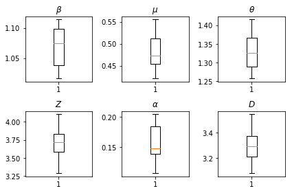
Wyniki naszych wnioskowań. Mamy wykreślić wartości największej wiarygodności dla wszystkich globalnych paramters pokazać ich zmienność w poprzek naszych num_batches niezależne przebiegi wnioskowania. Odpowiada to tabeli S1 w materiałach uzupełniających.
fig, axs = plt.subplots(2, 3)
axs[0, 0].boxplot(best_parameters.documented_infectious_tx_rate,
                  whis=(2.5,97.5), sym='')
axs[0, 0].set_title(r'$\beta$')

axs[0, 1].boxplot(best_parameters.undocumented_infectious_tx_relative_rate,
                  whis=(2.5,97.5), sym='')
axs[0, 1].set_title(r'$\mu$')

axs[0, 2].boxplot(best_parameters.intercity_underreporting_factor,
                  whis=(2.5,97.5), sym='')
axs[0, 2].set_title(r'$\theta$')

axs[1, 0].boxplot(best_parameters.average_latency_period,
                  whis=(2.5,97.5), sym='')
axs[1, 0].set_title(r'$Z$')

axs[1, 1].boxplot(best_parameters.fraction_of_documented_infections,
                  whis=(2.5,97.5), sym='')
axs[1, 1].set_title(r'$\alpha$')

axs[1, 2].boxplot(best_parameters.average_infection_duration,
                  whis=(2.5,97.5), sym='')
axs[1, 2].set_title(r'$D$')
plt.tight_layout()