| | |  عرض المصدر على جيثب عرض المصدر على جيثب | |
يطبق هذا البرنامج التعليمي شبكة عصبية تلافيفية كمومية مبسطة (QCNN) ، وهي نظير كمي مقترح لشبكة عصبية تلافيفية كلاسيكية تكون أيضًا ثابتة متعدية .
يوضح هذا المثال كيفية اكتشاف خصائص معينة لمصدر البيانات الكمومية ، مثل مستشعر الكم أو محاكاة معقدة من جهاز. مصدر البيانات الكمومية هو حالة الكتلة التي قد تكون أو لا تحتوي على إثارة - ما سوف تتعلم QCNN اكتشافه (مجموعة البيانات المستخدمة في الورقة كانت تصنيف طور SPT).
يثبت
pip install tensorflow==2.7.0
تثبيت TensorFlow Quantum:
pip install tensorflow-quantum
# Update package resources to account for version changes.
import importlib, pkg_resources
importlib.reload(pkg_resources)
<module 'pkg_resources' from '/tmpfs/src/tf_docs_env/lib/python3.7/site-packages/pkg_resources/__init__.py'>
الآن قم باستيراد TensorFlow وتبعيات الوحدة النمطية:
import tensorflow as tf
import tensorflow_quantum as tfq

import cirq
import sympy
import numpy as np

# visualization tools
%matplotlib inline
import matplotlib.pyplot as plt
from cirq.contrib.svg import SVGCircuit
2022-02-04 12:43:45.380301: E tensorflow/stream_executor/cuda/cuda_driver.cc:271] failed call to cuInit: CUDA_ERROR_NO_DEVICE: no CUDA-capable device is detected
1. بناء QCNN
1.1 تجميع الدوائر في رسم بياني TensorFlow
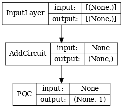
يوفر TensorFlow Quantum (TFQ) فئات طبقات مصممة لبناء الدوائر في الرسم البياني. أحد الأمثلة على ذلك هو طبقة tfq.layers.AddCircuit التي ترث من طبقة tf.keras.Layer . يمكن لهذه الطبقة إما أن تلحق أو تلحق بدفعة إدخال الدوائر ، كما هو موضح في الشكل التالي.
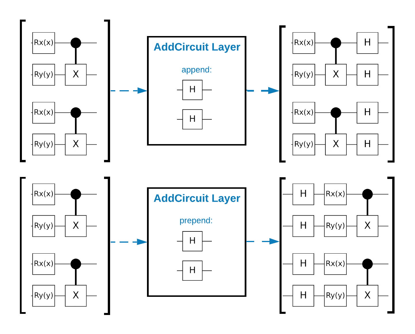
يستخدم المقتطف التالي هذه الطبقة:
qubit = cirq.GridQubit(0, 0)

# Define some circuits.
circuit1 = cirq.Circuit(cirq.X(qubit))
circuit2 = cirq.Circuit(cirq.H(qubit))

# Convert to a tensor.
input_circuit_tensor = tfq.convert_to_tensor([circuit1, circuit2])

# Define a circuit that we want to append
y_circuit = cirq.Circuit(cirq.Y(qubit))

# Instantiate our layer
y_appender = tfq.layers.AddCircuit()

# Run our circuit tensor through the layer and save the output.
output_circuit_tensor = y_appender(input_circuit_tensor, append=y_circuit)
افحص موتر الإدخال:
print(tfq.from_tensor(input_circuit_tensor))
[cirq.Circuit([
     cirq.Moment(
         cirq.X(cirq.GridQubit(0, 0)),
     ),
 ])
 cirq.Circuit([
     cirq.Moment(
         cirq.H(cirq.GridQubit(0, 0)),
     ),
 ])                                   ]
وفحص موتر الإخراج:
print(tfq.from_tensor(output_circuit_tensor))
[cirq.Circuit([
     cirq.Moment(
         cirq.X(cirq.GridQubit(0, 0)),
     ),
     cirq.Moment(
         cirq.Y(cirq.GridQubit(0, 0)),
     ),
 ])
 cirq.Circuit([
     cirq.Moment(
         cirq.H(cirq.GridQubit(0, 0)),
     ),
     cirq.Moment(
         cirq.Y(cirq.GridQubit(0, 0)),
     ),
 ])                                   ]
في حين أنه من الممكن تشغيل الأمثلة أدناه دون استخدام tfq.layers.AddCircuit ، فإنها فرصة جيدة لفهم كيف يمكن تضمين الوظائف المعقدة في الرسوم البيانية لحساب TensorFlow.
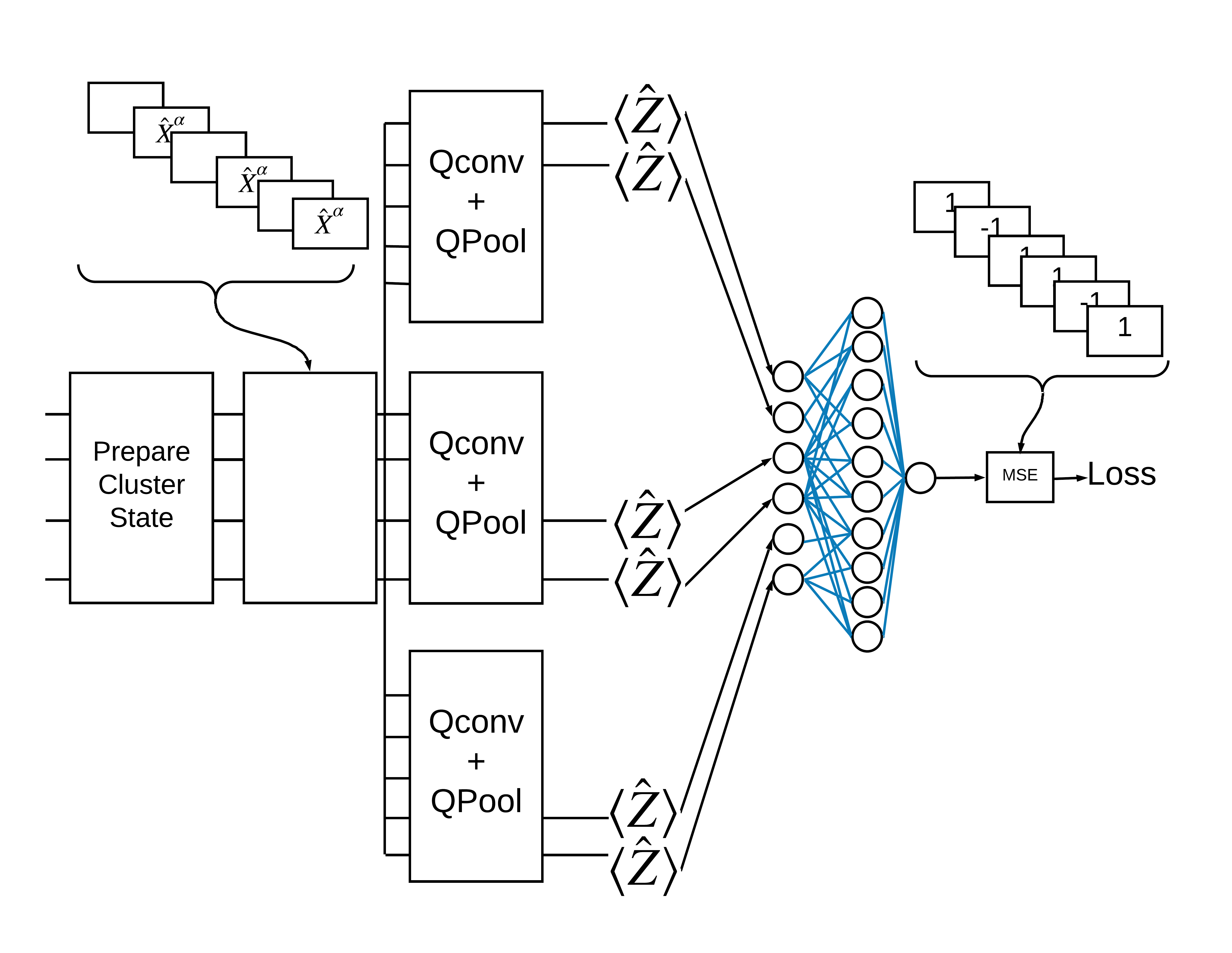
1.2 نظرة عامة على المشكلة
ستقوم بإعداد حالة الكتلة وتدريب المصنف الكمي لاكتشاف ما إذا كان "متحمسًا" أم لا. حالة الكتلة متشابكة للغاية ولكن ليس بالضرورة صعبًا على جهاز كمبيوتر كلاسيكي. من أجل الوضوح ، هذه مجموعة بيانات أبسط من تلك المستخدمة في الورق.
بالنسبة لمهمة التصنيف هذه ، ستقوم بتنفيذ بنية QCNN عميقة تشبه MERA منذ:
- مثل QCNN ، فإن حالة الكتلة على الحلقة ثابتة متعدية.
- حالة الكتلة متشابكة للغاية.
يجب أن تكون هذه البنية فعالة في تقليل التشابك ، والحصول على التصنيف من خلال قراءة كيوبت واحد.
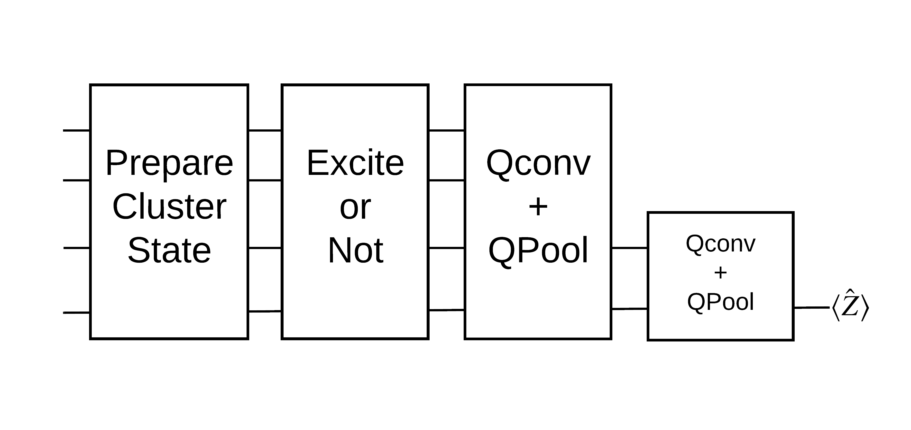
تُعرَّف حالة الكتلة "المستثارة" بأنها حالة الكتلة التي لها بوابة cirq.rx مطبقة على أي من الكيوبتات الخاصة بها. تمت مناقشة Qconv و QPool لاحقًا في هذا البرنامج التعليمي.
1.3 اللبنات الأساسية لـ TensorFlow
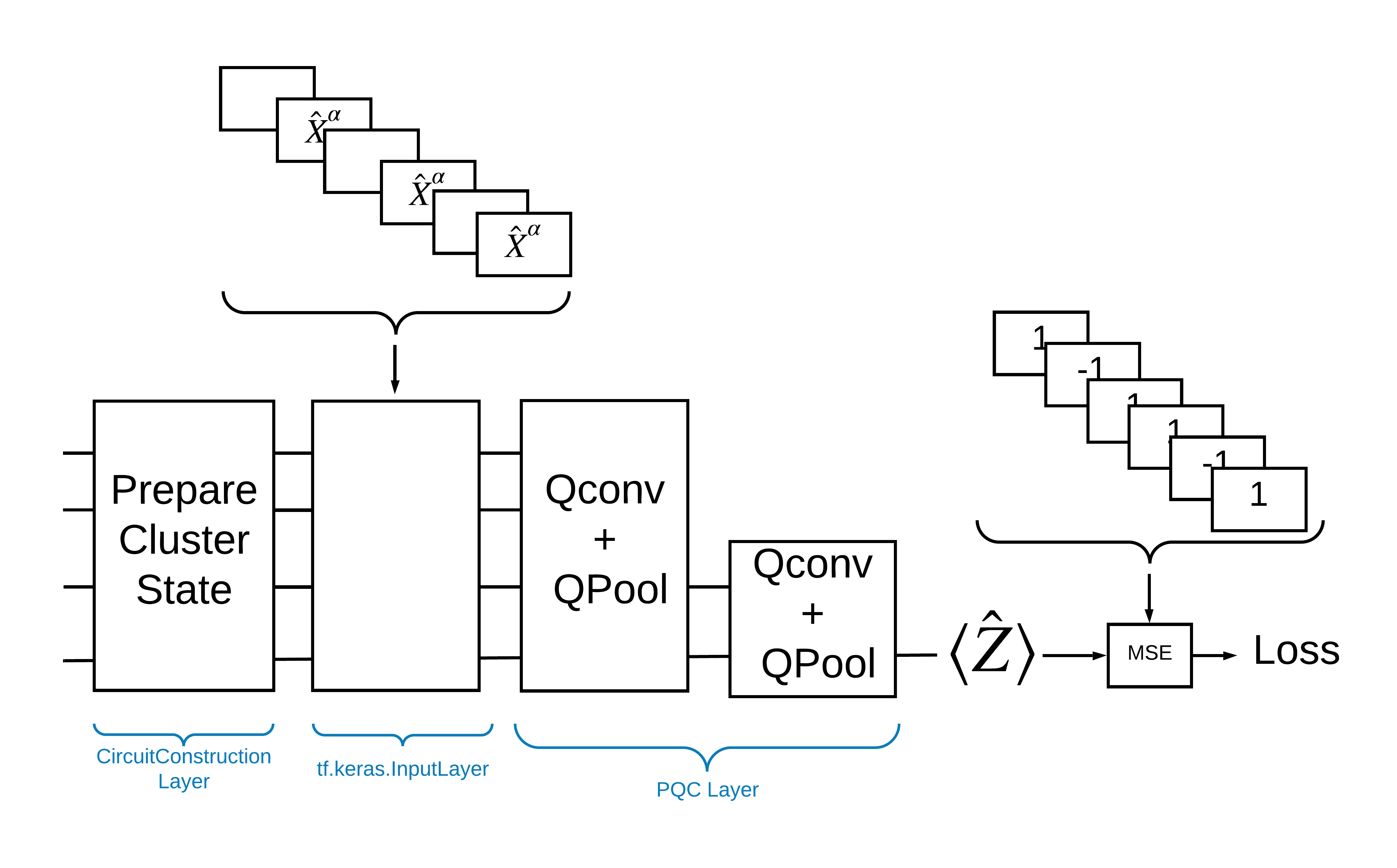
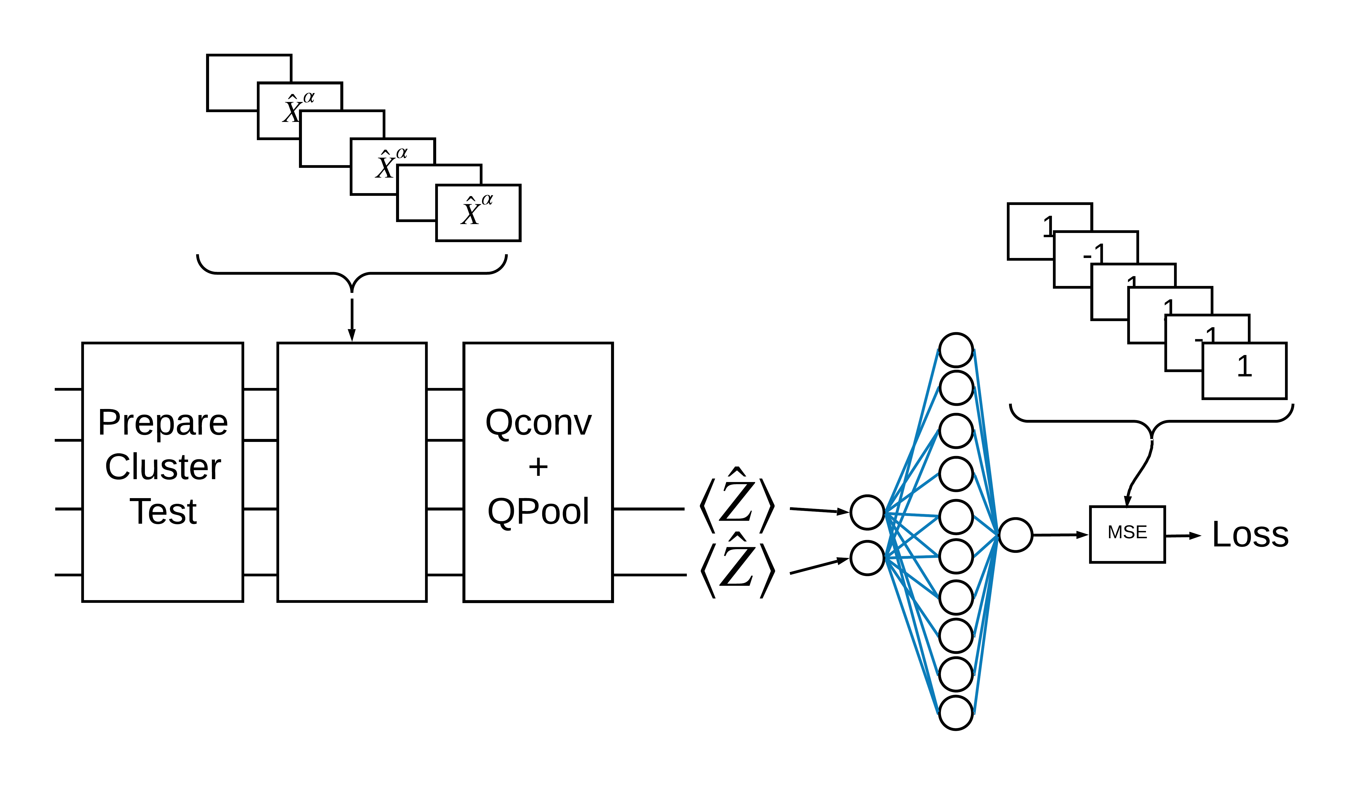
تتمثل إحدى طرق حل هذه المشكلة باستخدام TensorFlow Quantum في تنفيذ ما يلي:
- المدخل إلى النموذج هو موتر دارة - إما دائرة فارغة أو بوابة X على كيوبت معين يشير إلى الإثارة.
- يتم إنشاء باقي المكونات الكمومية للنموذج باستخدام طبقات
tfq.layers.AddCircuit. - للاستدلال ، يتم استخدام طبقة
tfq.layers.PQC. هذا يقرأ \(\langle \hat{Z} \rangle\) ويقارنه بتسمية 1 لحالة متحمس ، أو -1 لحالة غير متحمس.
1.4 البيانات
قبل بناء النموذج الخاص بك ، يمكنك إنشاء البيانات الخاصة بك. في هذه الحالة ، سيكون الأمر بمثابة إثارة لحالة الكتلة (تستخدم الورقة الأصلية مجموعة بيانات أكثر تعقيدًا). يتم تمثيل الإثارة cirq.rx يعتبر الدوران الكبير بدرجة كافية بمثابة إثارة ويتم تصنيفها على أنها 1 والدوران غير الكبير بدرجة كافية يتم تسميته -1 ولا يعتبر إثارة.
def generate_data(qubits):
    """Generate training and testing data."""
    n_rounds = 20  # Produces n_rounds * n_qubits datapoints.
    excitations = []
    labels = []
    for n in range(n_rounds):
        for bit in qubits:
            rng = np.random.uniform(-np.pi, np.pi)
            excitations.append(cirq.Circuit(cirq.rx(rng)(bit)))
            labels.append(1 if (-np.pi / 2) <= rng <= (np.pi / 2) else -1)

    split_ind = int(len(excitations) * 0.7)
    train_excitations = excitations[:split_ind]
    test_excitations = excitations[split_ind:]

    train_labels = labels[:split_ind]
    test_labels = labels[split_ind:]

    return tfq.convert_to_tensor(train_excitations), np.array(train_labels), \
        tfq.convert_to_tensor(test_excitations), np.array(test_labels)
يمكنك أن ترى أنه تمامًا كما هو الحال مع التعلم الآلي العادي ، يمكنك إنشاء مجموعة تدريب واختبار لاستخدامها في قياس النموذج. يمكنك إلقاء نظرة سريعة على بعض نقاط البيانات باستخدام:
sample_points, sample_labels, _, __ = generate_data(cirq.GridQubit.rect(1, 4))
print('Input:', tfq.from_tensor(sample_points)[0], 'Output:', sample_labels[0])
print('Input:', tfq.from_tensor(sample_points)[1], 'Output:', sample_labels[1])
Input: (0, 0): ───X^0.449─── Output: 1
Input: (0, 1): ───X^-0.74─── Output: -1
1.5 تحديد الطبقات
حدد الآن الطبقات الموضحة في الشكل أعلاه في TensorFlow.
1.5.1 حالة الكتلة
تتمثل الخطوة الأولى في تحديد حالة الكتلة باستخدام Cirq ، وهو إطار عمل مقدم من Google لبرمجة الدوائر الكمية. نظرًا لأن هذا جزء ثابت من النموذج ، قم بتضمينه باستخدام وظيفة tfq.layers.AddCircuit .
def cluster_state_circuit(bits):
    """Return a cluster state on the qubits in `bits`."""
    circuit = cirq.Circuit()
    circuit.append(cirq.H.on_each(bits))
    for this_bit, next_bit in zip(bits, bits[1:] + [bits[0]]):
        circuit.append(cirq.CZ(this_bit, next_bit))
    return circuit
عرض دائرة حالة الكتلة cirq.GridQubit s:
SVGCircuit(cluster_state_circuit(cirq.GridQubit.rect(1, 4)))
findfont: Font family ['Arial'] not found. Falling back to DejaVu Sans.

1.5.2 طبقات QCNN
حدد الطبقات التي يتكون منها النموذج باستخدام ورق Cong و Lukin QCNN . هناك بعض المتطلبات الأساسية:
- المصفوفات الوحدوية ذات المعلمات واحد واثنين كيوبت من ورقة Tucci .
- عملية تجميع ذات معلمات عامة ثنائية كيوبت.
def one_qubit_unitary(bit, symbols):
    """Make a Cirq circuit enacting a rotation of the bloch sphere about the X,
    Y and Z axis, that depends on the values in `symbols`.
    """
    return cirq.Circuit(
        cirq.X(bit)**symbols[0],
        cirq.Y(bit)**symbols[1],
        cirq.Z(bit)**symbols[2])


def two_qubit_unitary(bits, symbols):
    """Make a Cirq circuit that creates an arbitrary two qubit unitary."""
    circuit = cirq.Circuit()
    circuit += one_qubit_unitary(bits[0], symbols[0:3])
    circuit += one_qubit_unitary(bits[1], symbols[3:6])
    circuit += [cirq.ZZ(*bits)**symbols[6]]
    circuit += [cirq.YY(*bits)**symbols[7]]
    circuit += [cirq.XX(*bits)**symbols[8]]
    circuit += one_qubit_unitary(bits[0], symbols[9:12])
    circuit += one_qubit_unitary(bits[1], symbols[12:])
    return circuit


def two_qubit_pool(source_qubit, sink_qubit, symbols):
    """Make a Cirq circuit to do a parameterized 'pooling' operation, which
    attempts to reduce entanglement down from two qubits to just one."""
    pool_circuit = cirq.Circuit()
    sink_basis_selector = one_qubit_unitary(sink_qubit, symbols[0:3])
    source_basis_selector = one_qubit_unitary(source_qubit, symbols[3:6])
    pool_circuit.append(sink_basis_selector)
    pool_circuit.append(source_basis_selector)
    pool_circuit.append(cirq.CNOT(control=source_qubit, target=sink_qubit))
    pool_circuit.append(sink_basis_selector**-1)
    return pool_circuit
لترى ما قمت بإنشائه ، اطبع الدائرة الأحادية المكونة من كيوبت واحد:
SVGCircuit(one_qubit_unitary(cirq.GridQubit(0, 0), sympy.symbols('x0:3')))

والدائرة الوحدوية ثنائية البتات:
SVGCircuit(two_qubit_unitary(cirq.GridQubit.rect(1, 2), sympy.symbols('x0:15')))

ودائرة التجميع ثنائية الكوبت:
SVGCircuit(two_qubit_pool(*cirq.GridQubit.rect(1, 2), sympy.symbols('x0:6')))

1.5.2.1 الالتواء الكمي
كما هو الحال في ورقة Cong and Lukin ، حدد الالتواء الكمي أحادي الأبعاد باعتباره تطبيقًا لوحدة معيارية ذات معلمتين كيوبت على كل زوج من الكيوبتات المجاورة بخطوة واحدة.
def quantum_conv_circuit(bits, symbols):
    """Quantum Convolution Layer following the above diagram.
    Return a Cirq circuit with the cascade of `two_qubit_unitary` applied
    to all pairs of qubits in `bits` as in the diagram above.
    """
    circuit = cirq.Circuit()
    for first, second in zip(bits[0::2], bits[1::2]):
        circuit += two_qubit_unitary([first, second], symbols)
    for first, second in zip(bits[1::2], bits[2::2] + [bits[0]]):
        circuit += two_qubit_unitary([first, second], symbols)
    return circuit
اعرض الدائرة (الأفقية جدًا):
SVGCircuit(
    quantum_conv_circuit(cirq.GridQubit.rect(1, 8), sympy.symbols('x0:15')))

1.5.2.2 تجميع الكم
تجمعات طبقة تجميع الكم من \(N\) كيوبت إلى \(\frac{N}{2}\) كيوبت باستخدام تجمع 2 كيوبت المحدد أعلاه.
def quantum_pool_circuit(source_bits, sink_bits, symbols):
    """A layer that specifies a quantum pooling operation.
    A Quantum pool tries to learn to pool the relevant information from two
    qubits onto 1.
    """
    circuit = cirq.Circuit()
    for source, sink in zip(source_bits, sink_bits):
        circuit += two_qubit_pool(source, sink, symbols)
    return circuit
افحص دائرة مكون التجميع:
test_bits = cirq.GridQubit.rect(1, 8)

SVGCircuit(
    quantum_pool_circuit(test_bits[:4], test_bits[4:], sympy.symbols('x0:6')))

1.6 تعريف النموذج
الآن استخدم الطبقات المحددة لبناء شبكة CNN الكمومية البحتة. ابدأ بثمانية كيوبتات ، واجمعها لأسفل حتى تصل إلى واحد ، ثم \(\langle \hat{Z} \rangle\).
def create_model_circuit(qubits):
    """Create sequence of alternating convolution and pooling operators
    which gradually shrink over time."""
    model_circuit = cirq.Circuit()
    symbols = sympy.symbols('qconv0:63')
    # Cirq uses sympy.Symbols to map learnable variables. TensorFlow Quantum
    # scans incoming circuits and replaces these with TensorFlow variables.
    model_circuit += quantum_conv_circuit(qubits, symbols[0:15])
    model_circuit += quantum_pool_circuit(qubits[:4], qubits[4:],
                                          symbols[15:21])
    model_circuit += quantum_conv_circuit(qubits[4:], symbols[21:36])
    model_circuit += quantum_pool_circuit(qubits[4:6], qubits[6:],
                                          symbols[36:42])
    model_circuit += quantum_conv_circuit(qubits[6:], symbols[42:57])
    model_circuit += quantum_pool_circuit([qubits[6]], [qubits[7]],
                                          symbols[57:63])
    return model_circuit


# Create our qubits and readout operators in Cirq.
cluster_state_bits = cirq.GridQubit.rect(1, 8)
readout_operators = cirq.Z(cluster_state_bits[-1])

# Build a sequential model enacting the logic in 1.3 of this notebook.
# Here you are making the static cluster state prep as a part of the AddCircuit and the
# "quantum datapoints" are coming in the form of excitation
excitation_input = tf.keras.Input(shape=(), dtype=tf.dtypes.string)
cluster_state = tfq.layers.AddCircuit()(
    excitation_input, prepend=cluster_state_circuit(cluster_state_bits))

quantum_model = tfq.layers.PQC(create_model_circuit(cluster_state_bits),
                               readout_operators)(cluster_state)

qcnn_model = tf.keras.Model(inputs=[excitation_input], outputs=[quantum_model])

# Show the keras plot of the model
tf.keras.utils.plot_model(qcnn_model,
                          show_shapes=True,
                          show_layer_names=False,
                          dpi=70)
1.7 تدريب النموذج
قم بتدريب النموذج على الدفعة الكاملة لتبسيط هذا المثال.
# Generate some training data.
train_excitations, train_labels, test_excitations, test_labels = generate_data(
    cluster_state_bits)


# Custom accuracy metric.
@tf.function
def custom_accuracy(y_true, y_pred):
    y_true = tf.squeeze(y_true)
    y_pred = tf.map_fn(lambda x: 1.0 if x >= 0 else -1.0, y_pred)
    return tf.keras.backend.mean(tf.keras.backend.equal(y_true, y_pred))


qcnn_model.compile(optimizer=tf.keras.optimizers.Adam(learning_rate=0.02),
                   loss=tf.losses.mse,
                   metrics=[custom_accuracy])

history = qcnn_model.fit(x=train_excitations,
                         y=train_labels,
                         batch_size=16,
                         epochs=25,
                         verbose=1,
                         validation_data=(test_excitations, test_labels))
Epoch 1/25
7/7 [==============================] - 2s 176ms/step - loss: 0.8961 - custom_accuracy: 0.7143 - val_loss: 0.8012 - val_custom_accuracy: 0.7500
Epoch 2/25
7/7 [==============================] - 1s 140ms/step - loss: 0.7736 - custom_accuracy: 0.7946 - val_loss: 0.7355 - val_custom_accuracy: 0.8542
Epoch 3/25
7/7 [==============================] - 1s 138ms/step - loss: 0.7319 - custom_accuracy: 0.8393 - val_loss: 0.7045 - val_custom_accuracy: 0.8125
Epoch 4/25
7/7 [==============================] - 1s 137ms/step - loss: 0.6976 - custom_accuracy: 0.8482 - val_loss: 0.6829 - val_custom_accuracy: 0.8333
Epoch 5/25
7/7 [==============================] - 1s 143ms/step - loss: 0.6696 - custom_accuracy: 0.8750 - val_loss: 0.6749 - val_custom_accuracy: 0.7917
Epoch 6/25
7/7 [==============================] - 1s 137ms/step - loss: 0.6631 - custom_accuracy: 0.8750 - val_loss: 0.6718 - val_custom_accuracy: 0.7917
Epoch 7/25
7/7 [==============================] - 1s 135ms/step - loss: 0.6536 - custom_accuracy: 0.8929 - val_loss: 0.6638 - val_custom_accuracy: 0.8750
Epoch 8/25
7/7 [==============================] - 1s 141ms/step - loss: 0.6376 - custom_accuracy: 0.8750 - val_loss: 0.6311 - val_custom_accuracy: 0.8542
Epoch 9/25
7/7 [==============================] - 1s 137ms/step - loss: 0.6208 - custom_accuracy: 0.8750 - val_loss: 0.5995 - val_custom_accuracy: 0.8542
Epoch 10/25
7/7 [==============================] - 1s 134ms/step - loss: 0.5887 - custom_accuracy: 0.8661 - val_loss: 0.5655 - val_custom_accuracy: 0.8333
Epoch 11/25
7/7 [==============================] - 1s 144ms/step - loss: 0.5796 - custom_accuracy: 0.8482 - val_loss: 0.5681 - val_custom_accuracy: 0.8333
Epoch 12/25
7/7 [==============================] - 1s 143ms/step - loss: 0.5630 - custom_accuracy: 0.7946 - val_loss: 0.5179 - val_custom_accuracy: 0.8333
Epoch 13/25
7/7 [==============================] - 1s 137ms/step - loss: 0.5405 - custom_accuracy: 0.8304 - val_loss: 0.5003 - val_custom_accuracy: 0.8333
Epoch 14/25
7/7 [==============================] - 1s 138ms/step - loss: 0.5259 - custom_accuracy: 0.8036 - val_loss: 0.4787 - val_custom_accuracy: 0.8333
Epoch 15/25
7/7 [==============================] - 1s 137ms/step - loss: 0.5077 - custom_accuracy: 0.8482 - val_loss: 0.4741 - val_custom_accuracy: 0.8125
Epoch 16/25
7/7 [==============================] - 1s 136ms/step - loss: 0.5082 - custom_accuracy: 0.8214 - val_loss: 0.4739 - val_custom_accuracy: 0.8125
Epoch 17/25
7/7 [==============================] - 1s 137ms/step - loss: 0.5138 - custom_accuracy: 0.8214 - val_loss: 0.4859 - val_custom_accuracy: 0.8750
Epoch 18/25
7/7 [==============================] - 1s 133ms/step - loss: 0.5073 - custom_accuracy: 0.8304 - val_loss: 0.4879 - val_custom_accuracy: 0.8333
Epoch 19/25
7/7 [==============================] - 1s 138ms/step - loss: 0.5084 - custom_accuracy: 0.8304 - val_loss: 0.4745 - val_custom_accuracy: 0.8542
Epoch 20/25
7/7 [==============================] - 1s 139ms/step - loss: 0.5057 - custom_accuracy: 0.8571 - val_loss: 0.4702 - val_custom_accuracy: 0.8333
Epoch 21/25
7/7 [==============================] - 1s 135ms/step - loss: 0.4939 - custom_accuracy: 0.8304 - val_loss: 0.4734 - val_custom_accuracy: 0.8750
Epoch 22/25
7/7 [==============================] - 1s 138ms/step - loss: 0.4942 - custom_accuracy: 0.8750 - val_loss: 0.4725 - val_custom_accuracy: 0.8750
Epoch 23/25
7/7 [==============================] - 1s 140ms/step - loss: 0.4982 - custom_accuracy: 0.9107 - val_loss: 0.4695 - val_custom_accuracy: 0.8958
Epoch 24/25
7/7 [==============================] - 1s 135ms/step - loss: 0.4936 - custom_accuracy: 0.8661 - val_loss: 0.4731 - val_custom_accuracy: 0.8750
Epoch 25/25
7/7 [==============================] - 1s 136ms/step - loss: 0.4866 - custom_accuracy: 0.8571 - val_loss: 0.4631 - val_custom_accuracy: 0.8958
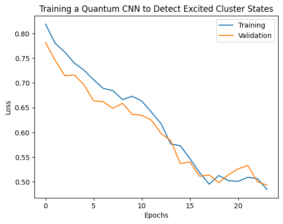
plt.plot(history.history['loss'][1:], label='Training')
plt.plot(history.history['val_loss'][1:], label='Validation')
plt.title('Training a Quantum CNN to Detect Excited Cluster States')
plt.xlabel('Epochs')
plt.ylabel('Loss')
plt.legend()
plt.show()
2. النماذج الهجينة
لست مضطرًا للانتقال من ثمانية كيوبتات إلى كيوبت واحد باستخدام الالتواء الكمي - كان بإمكانك القيام بجولة أو جولتين من الالتواء الكمومي وإدخال النتائج في شبكة عصبية كلاسيكية. يستكشف هذا القسم النماذج الهجينة الكلاسيكية الكم.
2.1 نموذج هجين مع مرشح كمي واحد
طبق طبقة واحدة من الالتواء الكمومي ، \(\langle \hat{Z}_n \rangle\) على جميع البتات ، متبوعًا بشبكة عصبية متصلة بكثافة.
2.1.1 تعريف النموذج
# 1-local operators to read out
readouts = [cirq.Z(bit) for bit in cluster_state_bits[4:]]
def multi_readout_model_circuit(qubits):
"""Make a model circuit with less quantum pool and conv operations."""
model_circuit = cirq.Circuit()
symbols = sympy.symbols('qconv0:21')
model_circuit += quantum_conv_circuit(qubits, symbols[0:15])
model_circuit += quantum_pool_circuit(qubits[:4], qubits[4:],
symbols[15:21])
return model_circuit
# Build a model enacting the logic in 2.1 of this notebook.
excitation_input_dual = tf.keras.Input(shape=(), dtype=tf.dtypes.string)
cluster_state_dual = tfq.layers.AddCircuit()(
excitation_input_dual, prepend=cluster_state_circuit(cluster_state_bits))
quantum_model_dual = tfq.layers.PQC(
multi_readout_model_circuit(cluster_state_bits),
readouts)(cluster_state_dual)
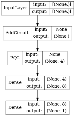
d1_dual = tf.keras.layers.Dense(8)(quantum_model_dual)
d2_dual = tf.keras.layers.Dense(1)(d1_dual)
hybrid_model = tf.keras.Model(inputs=[excitation_input_dual], outputs=[d2_dual])
# Display the model architecture
tf.keras.utils.plot_model(hybrid_model,
show_shapes=True,
show_layer_names=False,
dpi=70)
2.1.2 تدريب النموذج
hybrid_model.compile(optimizer=tf.keras.optimizers.Adam(learning_rate=0.02),
                     loss=tf.losses.mse,
                     metrics=[custom_accuracy])

hybrid_history = hybrid_model.fit(x=train_excitations,
                                  y=train_labels,
                                  batch_size=16,
                                  epochs=25,
                                  verbose=1,
                                  validation_data=(test_excitations,
                                                   test_labels))
Epoch 1/25
7/7 [==============================] - 1s 113ms/step - loss: 0.9848 - custom_accuracy: 0.5179 - val_loss: 0.9635 - val_custom_accuracy: 0.5417
Epoch 2/25
7/7 [==============================] - 1s 86ms/step - loss: 0.8095 - custom_accuracy: 0.6339 - val_loss: 0.6800 - val_custom_accuracy: 0.7083
Epoch 3/25
7/7 [==============================] - 1s 85ms/step - loss: 0.4045 - custom_accuracy: 0.9375 - val_loss: 0.3342 - val_custom_accuracy: 0.8750
Epoch 4/25
7/7 [==============================] - 1s 86ms/step - loss: 0.2308 - custom_accuracy: 0.9643 - val_loss: 0.2027 - val_custom_accuracy: 0.9792
Epoch 5/25
7/7 [==============================] - 1s 84ms/step - loss: 0.2232 - custom_accuracy: 0.9554 - val_loss: 0.1761 - val_custom_accuracy: 1.0000
Epoch 6/25
7/7 [==============================] - 1s 84ms/step - loss: 0.1760 - custom_accuracy: 0.9821 - val_loss: 0.2541 - val_custom_accuracy: 0.9167
Epoch 7/25
7/7 [==============================] - 1s 85ms/step - loss: 0.1919 - custom_accuracy: 0.9643 - val_loss: 0.1967 - val_custom_accuracy: 0.9792
Epoch 8/25
7/7 [==============================] - 1s 83ms/step - loss: 0.1892 - custom_accuracy: 0.9554 - val_loss: 0.1870 - val_custom_accuracy: 0.9792
Epoch 9/25
7/7 [==============================] - 1s 84ms/step - loss: 0.1777 - custom_accuracy: 0.9911 - val_loss: 0.2208 - val_custom_accuracy: 0.9583
Epoch 10/25
7/7 [==============================] - 1s 83ms/step - loss: 0.1728 - custom_accuracy: 0.9732 - val_loss: 0.2147 - val_custom_accuracy: 0.9583
Epoch 11/25
7/7 [==============================] - 1s 85ms/step - loss: 0.1704 - custom_accuracy: 0.9732 - val_loss: 0.1810 - val_custom_accuracy: 0.9792
Epoch 12/25
7/7 [==============================] - 1s 85ms/step - loss: 0.1739 - custom_accuracy: 0.9732 - val_loss: 0.2038 - val_custom_accuracy: 0.9792
Epoch 13/25
7/7 [==============================] - 1s 81ms/step - loss: 0.1705 - custom_accuracy: 0.9732 - val_loss: 0.1855 - val_custom_accuracy: 0.9792
Epoch 14/25
7/7 [==============================] - 1s 84ms/step - loss: 0.1788 - custom_accuracy: 0.9643 - val_loss: 0.2152 - val_custom_accuracy: 0.9583
Epoch 15/25
7/7 [==============================] - 1s 84ms/step - loss: 0.1760 - custom_accuracy: 0.9732 - val_loss: 0.1994 - val_custom_accuracy: 1.0000
Epoch 16/25
7/7 [==============================] - 1s 83ms/step - loss: 0.1737 - custom_accuracy: 0.9732 - val_loss: 0.2035 - val_custom_accuracy: 0.9792
Epoch 17/25
7/7 [==============================] - 1s 82ms/step - loss: 0.1749 - custom_accuracy: 0.9911 - val_loss: 0.1983 - val_custom_accuracy: 0.9583
Epoch 18/25
7/7 [==============================] - 1s 83ms/step - loss: 0.1875 - custom_accuracy: 0.9732 - val_loss: 0.1916 - val_custom_accuracy: 0.9583
Epoch 19/25
7/7 [==============================] - 1s 82ms/step - loss: 0.1605 - custom_accuracy: 0.9732 - val_loss: 0.1782 - val_custom_accuracy: 0.9792
Epoch 20/25
7/7 [==============================] - 1s 84ms/step - loss: 0.1668 - custom_accuracy: 0.9911 - val_loss: 0.2276 - val_custom_accuracy: 0.9583
Epoch 21/25
7/7 [==============================] - 1s 84ms/step - loss: 0.1700 - custom_accuracy: 0.9911 - val_loss: 0.2080 - val_custom_accuracy: 0.9583
Epoch 22/25
7/7 [==============================] - 1s 83ms/step - loss: 0.1621 - custom_accuracy: 0.9732 - val_loss: 0.1851 - val_custom_accuracy: 0.9375
Epoch 23/25
7/7 [==============================] - 1s 84ms/step - loss: 0.1695 - custom_accuracy: 0.9911 - val_loss: 0.1882 - val_custom_accuracy: 0.9792
Epoch 24/25
7/7 [==============================] - 1s 82ms/step - loss: 0.1583 - custom_accuracy: 0.9911 - val_loss: 0.2017 - val_custom_accuracy: 0.9583
Epoch 25/25
7/7 [==============================] - 1s 83ms/step - loss: 0.1557 - custom_accuracy: 0.9911 - val_loss: 0.1907 - val_custom_accuracy: 0.9792
plt.plot(history.history['val_custom_accuracy'], label='QCNN')
plt.plot(hybrid_history.history['val_custom_accuracy'], label='Hybrid CNN')
plt.title('Quantum vs Hybrid CNN performance')
plt.xlabel('Epochs')
plt.legend()
plt.ylabel('Validation Accuracy')
plt.show()
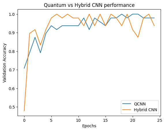
كما ترون ، بمساعدة كلاسيكية متواضعة للغاية ، عادةً ما يتقارب النموذج الهجين أسرع من الإصدار الكمي البحت.
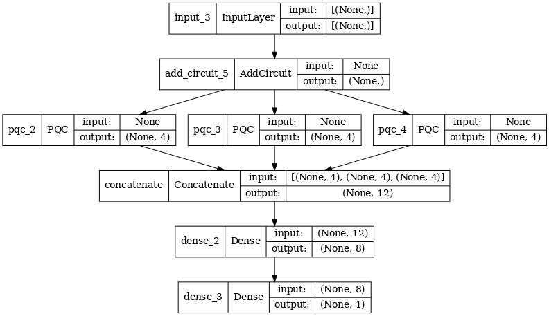
2.2 التفاف هجين مع مرشحات كمية متعددة
لنجرب الآن بنية تستخدم تلافيف كمومية متعددة وشبكة عصبية كلاسيكية لدمجها.
2.2.1 تعريف النموذج
excitation_input_multi = tf.keras.Input(shape=(), dtype=tf.dtypes.string)

cluster_state_multi = tfq.layers.AddCircuit()(
    excitation_input_multi, prepend=cluster_state_circuit(cluster_state_bits))

# apply 3 different filters and measure expectation values

quantum_model_multi1 = tfq.layers.PQC(
    multi_readout_model_circuit(cluster_state_bits),
    readouts)(cluster_state_multi)

quantum_model_multi2 = tfq.layers.PQC(
    multi_readout_model_circuit(cluster_state_bits),
    readouts)(cluster_state_multi)

quantum_model_multi3 = tfq.layers.PQC(
    multi_readout_model_circuit(cluster_state_bits),
    readouts)(cluster_state_multi)

# concatenate outputs and feed into a small classical NN
concat_out = tf.keras.layers.concatenate(
    [quantum_model_multi1, quantum_model_multi2, quantum_model_multi3])

dense_1 = tf.keras.layers.Dense(8)(concat_out)

dense_2 = tf.keras.layers.Dense(1)(dense_1)

multi_qconv_model = tf.keras.Model(inputs=[excitation_input_multi],
                                   outputs=[dense_2])

# Display the model architecture
tf.keras.utils.plot_model(multi_qconv_model,
                          show_shapes=True,
                          show_layer_names=True,
                          dpi=70)
2.2.2 تدريب النموذج
multi_qconv_model.compile(
    optimizer=tf.keras.optimizers.Adam(learning_rate=0.02),
    loss=tf.losses.mse,
    metrics=[custom_accuracy])

multi_qconv_history = multi_qconv_model.fit(x=train_excitations,
                                            y=train_labels,
                                            batch_size=16,
                                            epochs=25,
                                            verbose=1,
                                            validation_data=(test_excitations,
                                                             test_labels))
Epoch 1/25
7/7 [==============================] - 2s 143ms/step - loss: 0.9425 - custom_accuracy: 0.6429 - val_loss: 0.8120 - val_custom_accuracy: 0.7083
Epoch 2/25
7/7 [==============================] - 1s 109ms/step - loss: 0.5778 - custom_accuracy: 0.7946 - val_loss: 0.5920 - val_custom_accuracy: 0.7500
Epoch 3/25
7/7 [==============================] - 1s 103ms/step - loss: 0.4954 - custom_accuracy: 0.9018 - val_loss: 0.4568 - val_custom_accuracy: 0.7708
Epoch 4/25
7/7 [==============================] - 1s 95ms/step - loss: 0.2855 - custom_accuracy: 0.9196 - val_loss: 0.2792 - val_custom_accuracy: 0.9375
Epoch 5/25
7/7 [==============================] - 1s 93ms/step - loss: 0.1902 - custom_accuracy: 0.9821 - val_loss: 0.2212 - val_custom_accuracy: 0.9375
Epoch 6/25
7/7 [==============================] - 1s 94ms/step - loss: 0.1685 - custom_accuracy: 0.9821 - val_loss: 0.2341 - val_custom_accuracy: 0.9583
Epoch 7/25
7/7 [==============================] - 1s 104ms/step - loss: 0.1671 - custom_accuracy: 0.9911 - val_loss: 0.2062 - val_custom_accuracy: 0.9792
Epoch 8/25
7/7 [==============================] - 1s 97ms/step - loss: 0.1511 - custom_accuracy: 0.9821 - val_loss: 0.2096 - val_custom_accuracy: 0.9792
Epoch 9/25
7/7 [==============================] - 1s 96ms/step - loss: 0.1432 - custom_accuracy: 0.9911 - val_loss: 0.2330 - val_custom_accuracy: 0.9375
Epoch 10/25
7/7 [==============================] - 1s 92ms/step - loss: 0.1668 - custom_accuracy: 0.9821 - val_loss: 0.2344 - val_custom_accuracy: 0.9583
Epoch 11/25
7/7 [==============================] - 1s 106ms/step - loss: 0.1893 - custom_accuracy: 0.9732 - val_loss: 0.2148 - val_custom_accuracy: 0.9583
Epoch 12/25
7/7 [==============================] - 1s 104ms/step - loss: 0.1857 - custom_accuracy: 0.9732 - val_loss: 0.2739 - val_custom_accuracy: 0.9583
Epoch 13/25
7/7 [==============================] - 1s 106ms/step - loss: 0.1748 - custom_accuracy: 0.9732 - val_loss: 0.2366 - val_custom_accuracy: 0.9583
Epoch 14/25
7/7 [==============================] - 1s 103ms/step - loss: 0.1515 - custom_accuracy: 0.9821 - val_loss: 0.2012 - val_custom_accuracy: 0.9583
Epoch 15/25
7/7 [==============================] - 1s 100ms/step - loss: 0.1552 - custom_accuracy: 0.9911 - val_loss: 0.2404 - val_custom_accuracy: 0.9375
Epoch 16/25
7/7 [==============================] - 1s 97ms/step - loss: 0.1572 - custom_accuracy: 0.9911 - val_loss: 0.2779 - val_custom_accuracy: 0.9375
Epoch 17/25
7/7 [==============================] - 1s 100ms/step - loss: 0.1546 - custom_accuracy: 0.9821 - val_loss: 0.2104 - val_custom_accuracy: 0.9583
Epoch 18/25
7/7 [==============================] - 1s 102ms/step - loss: 0.1418 - custom_accuracy: 0.9911 - val_loss: 0.2647 - val_custom_accuracy: 0.9583
Epoch 19/25
7/7 [==============================] - 1s 98ms/step - loss: 0.1590 - custom_accuracy: 0.9732 - val_loss: 0.2154 - val_custom_accuracy: 0.9583
Epoch 20/25
7/7 [==============================] - 1s 104ms/step - loss: 0.1363 - custom_accuracy: 1.0000 - val_loss: 0.2470 - val_custom_accuracy: 0.9375
Epoch 21/25
7/7 [==============================] - 1s 100ms/step - loss: 0.1442 - custom_accuracy: 0.9821 - val_loss: 0.2383 - val_custom_accuracy: 0.9375
Epoch 22/25
7/7 [==============================] - 1s 99ms/step - loss: 0.1415 - custom_accuracy: 0.9911 - val_loss: 0.2324 - val_custom_accuracy: 0.9583
Epoch 23/25
7/7 [==============================] - 1s 97ms/step - loss: 0.1424 - custom_accuracy: 0.9821 - val_loss: 0.2188 - val_custom_accuracy: 0.9583
Epoch 24/25
7/7 [==============================] - 1s 100ms/step - loss: 0.1417 - custom_accuracy: 0.9821 - val_loss: 0.2340 - val_custom_accuracy: 0.9375
Epoch 25/25
7/7 [==============================] - 1s 103ms/step - loss: 0.1471 - custom_accuracy: 0.9732 - val_loss: 0.2252 - val_custom_accuracy: 0.9583
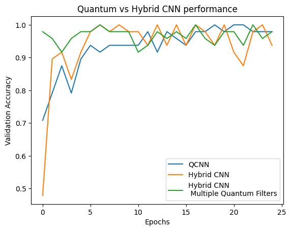
plt.plot(history.history['val_custom_accuracy'][:25], label='QCNN')
plt.plot(hybrid_history.history['val_custom_accuracy'][:25], label='Hybrid CNN')
plt.plot(multi_qconv_history.history['val_custom_accuracy'][:25],
         label='Hybrid CNN \n Multiple Quantum Filters')
plt.title('Quantum vs Hybrid CNN performance')
plt.xlabel('Epochs')
plt.legend()
plt.ylabel('Validation Accuracy')
plt.show()