| | |  Visualizza l'origine su GitHub Visualizza l'origine su GitHub | |
Questo tutorial implementa una rete neurale convoluzionale quantistica (QCNN) semplificata, un analogo quantistico proposto per una rete neurale convoluzionale classica che è anche traslazionalmente invariante .
Questo esempio mostra come rilevare determinate proprietà di un'origine dati quantistica, come un sensore quantistico o una simulazione complessa da un dispositivo. La fonte di dati quantistici è uno stato del cluster che può avere o meno un'eccitazione, ciò che la QCNN imparerà a rilevare (il set di dati utilizzato nel documento era la classificazione di fase SPT).
Impostare
pip install tensorflow==2.7.0
Installa TensorFlow Quantum:
pip install tensorflow-quantum
# Update package resources to account for version changes.
import importlib, pkg_resources
importlib.reload(pkg_resources)
<module 'pkg_resources' from '/tmpfs/src/tf_docs_env/lib/python3.7/site-packages/pkg_resources/__init__.py'>
Ora importa TensorFlow e le dipendenze del modulo:
import tensorflow as tf
import tensorflow_quantum as tfq

import cirq
import sympy
import numpy as np

# visualization tools
%matplotlib inline
import matplotlib.pyplot as plt
from cirq.contrib.svg import SVGCircuit
2022-02-04 12:43:45.380301: E tensorflow/stream_executor/cuda/cuda_driver.cc:271] failed call to cuInit: CUDA_ERROR_NO_DEVICE: no CUDA-capable device is detected
1. Costruisci una QCNN
1.1 Assemblare i circuiti in un grafico TensorFlow
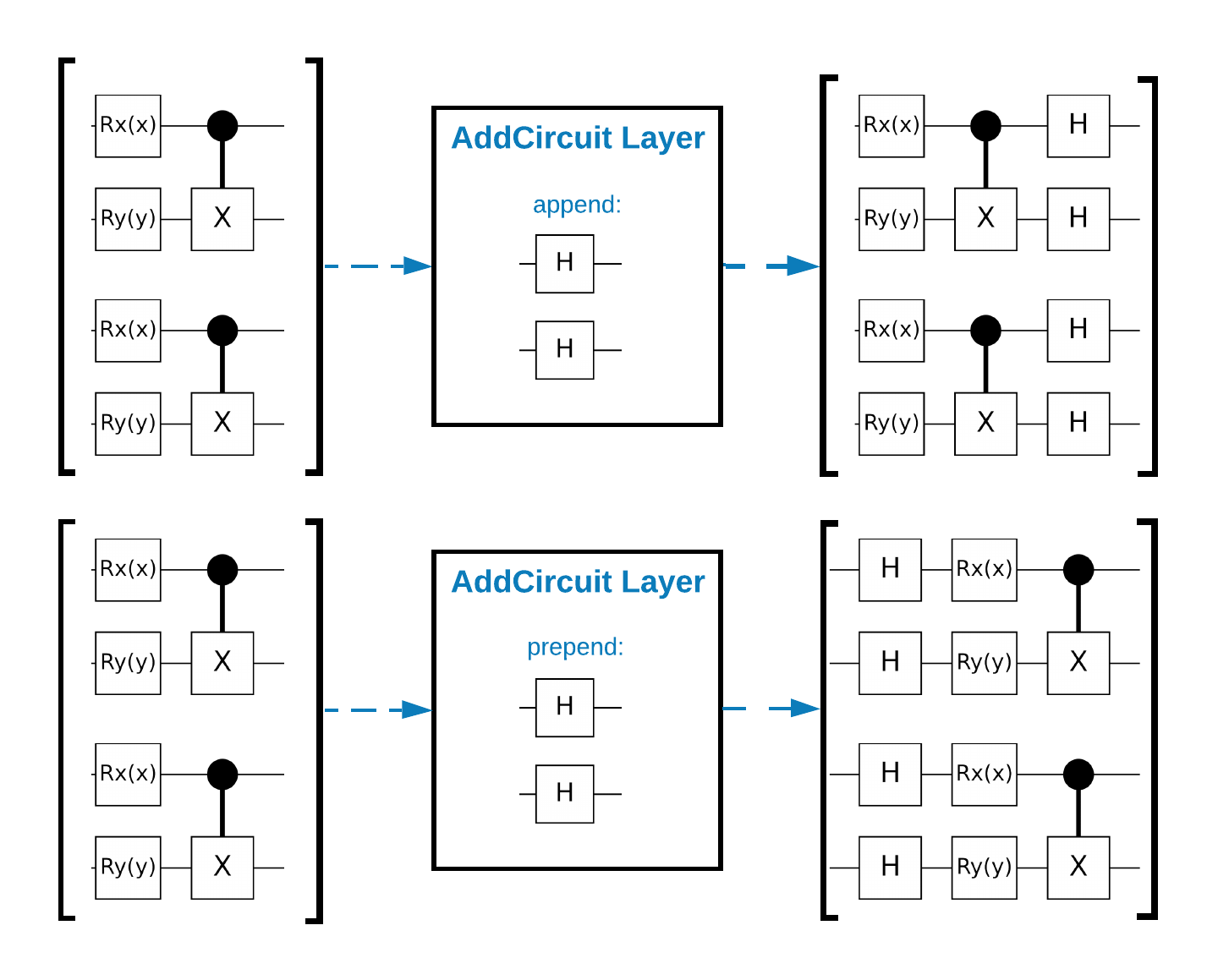
TensorFlow Quantum (TFQ) fornisce classi di livello progettate per la costruzione di circuiti in-graph. Un esempio è il livello tfq.layers.AddCircuit che eredita da tf.keras.Layer . Questo livello può essere anteposto o aggiunto al batch di circuiti di input, come mostrato nella figura seguente.
Il frammento di codice seguente utilizza questo livello:
qubit = cirq.GridQubit(0, 0)

# Define some circuits.
circuit1 = cirq.Circuit(cirq.X(qubit))
circuit2 = cirq.Circuit(cirq.H(qubit))

# Convert to a tensor.
input_circuit_tensor = tfq.convert_to_tensor([circuit1, circuit2])

# Define a circuit that we want to append
y_circuit = cirq.Circuit(cirq.Y(qubit))

# Instantiate our layer
y_appender = tfq.layers.AddCircuit()

# Run our circuit tensor through the layer and save the output.
output_circuit_tensor = y_appender(input_circuit_tensor, append=y_circuit)
Esamina il tensore di input:
print(tfq.from_tensor(input_circuit_tensor))
[cirq.Circuit([
     cirq.Moment(
         cirq.X(cirq.GridQubit(0, 0)),
     ),
 ])
 cirq.Circuit([
     cirq.Moment(
         cirq.H(cirq.GridQubit(0, 0)),
     ),
 ])                                   ]
Ed esamina il tensore di uscita:
print(tfq.from_tensor(output_circuit_tensor))
[cirq.Circuit([
     cirq.Moment(
         cirq.X(cirq.GridQubit(0, 0)),
     ),
     cirq.Moment(
         cirq.Y(cirq.GridQubit(0, 0)),
     ),
 ])
 cirq.Circuit([
     cirq.Moment(
         cirq.H(cirq.GridQubit(0, 0)),
     ),
     cirq.Moment(
         cirq.Y(cirq.GridQubit(0, 0)),
     ),
 ])                                   ]
Sebbene sia possibile eseguire gli esempi seguenti senza utilizzare tfq.layers.AddCircuit , è una buona opportunità per comprendere come funzionalità complesse possono essere incorporate nei grafici di calcolo TensorFlow.
1.2 Panoramica del problema
Preparerai uno stato del cluster e addestrerai un classificatore quantistico per rilevare se è "eccitato" o meno. Lo stato del cluster è altamente intrecciato ma non necessariamente difficile per un computer classico. Per chiarezza, questo è un set di dati più semplice di quello utilizzato nel documento.
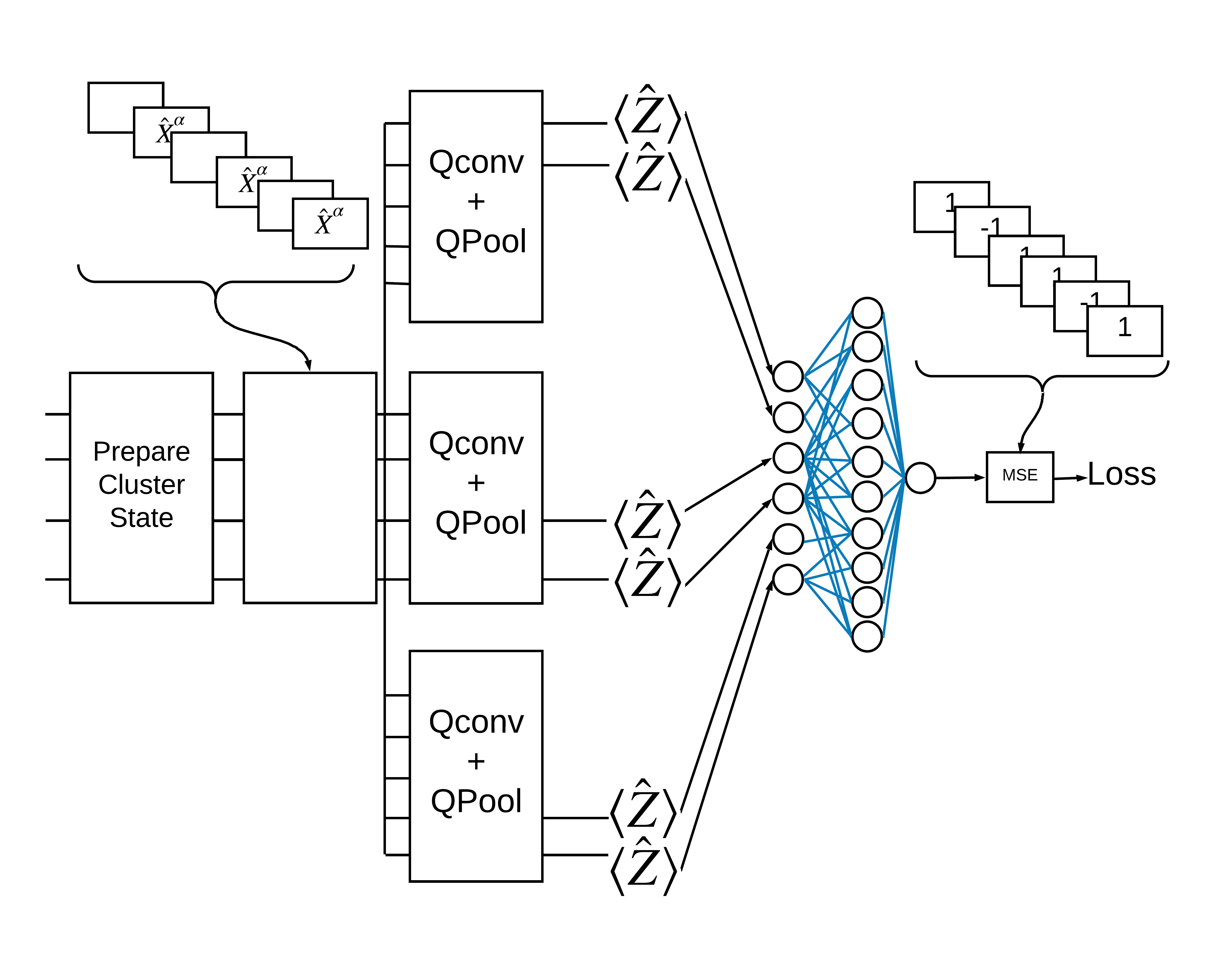
Per questa attività di classificazione implementerai un'architettura QCNN simile a MERA poiché:
- Come il QCNN, lo stato del cluster su un anello è traslazionale invariante.
- Lo stato del cluster è altamente intrecciato.
Questa architettura dovrebbe essere efficace nel ridurre l'entanglement, ottenendo la classificazione leggendo un singolo qubit.
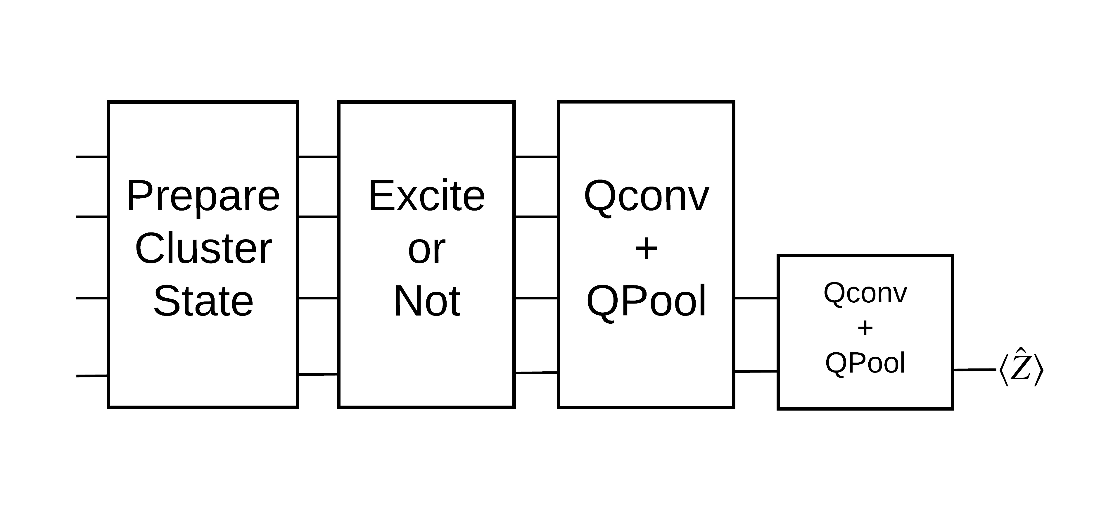
Uno stato del cluster "eccitato" è definito come uno stato del cluster a cui è stata applicata una porta cirq.rx a uno qualsiasi dei suoi qubit. Qconv e QPool sono discussi più avanti in questo tutorial.
1.3 Elementi costitutivi per TensorFlow
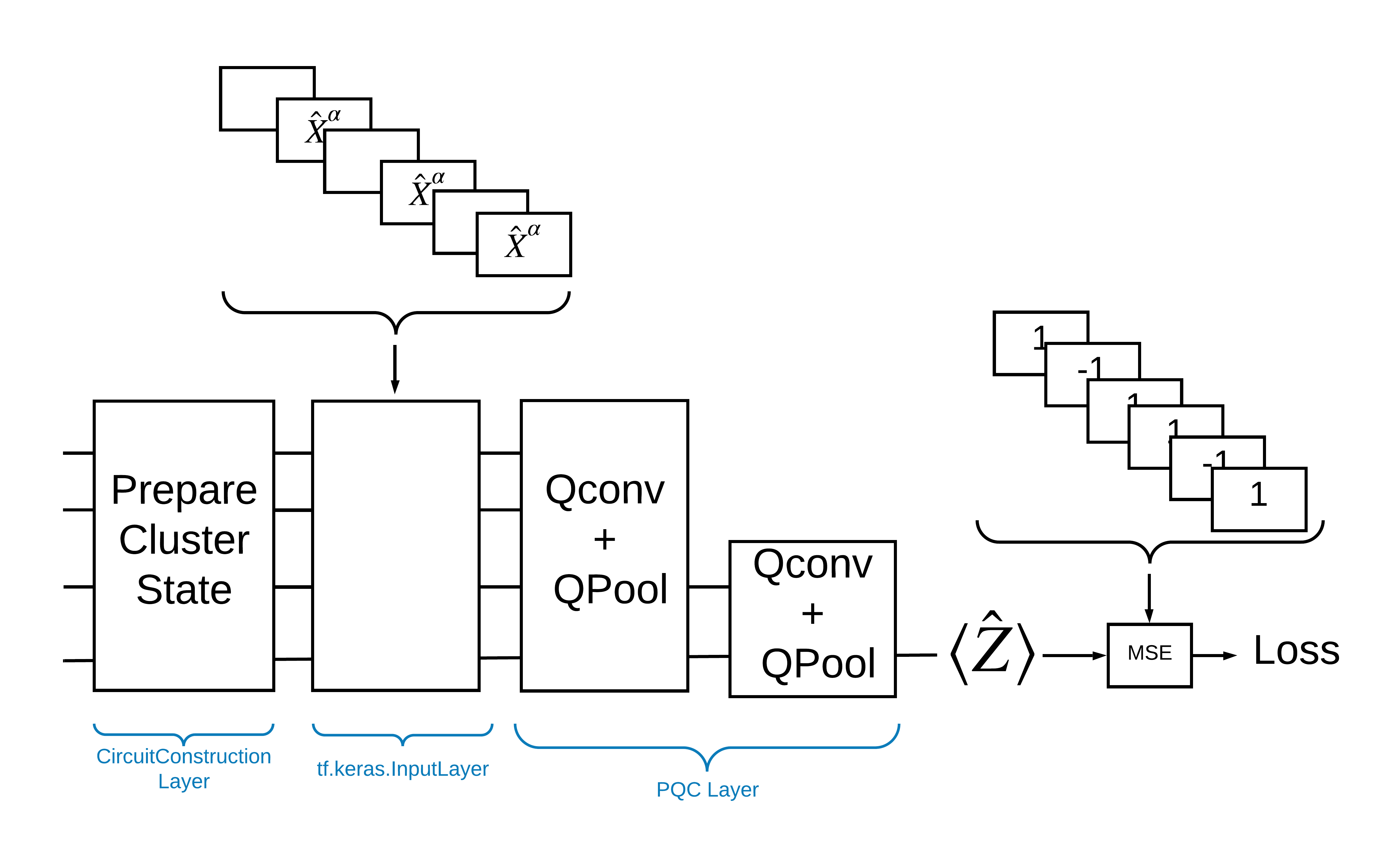
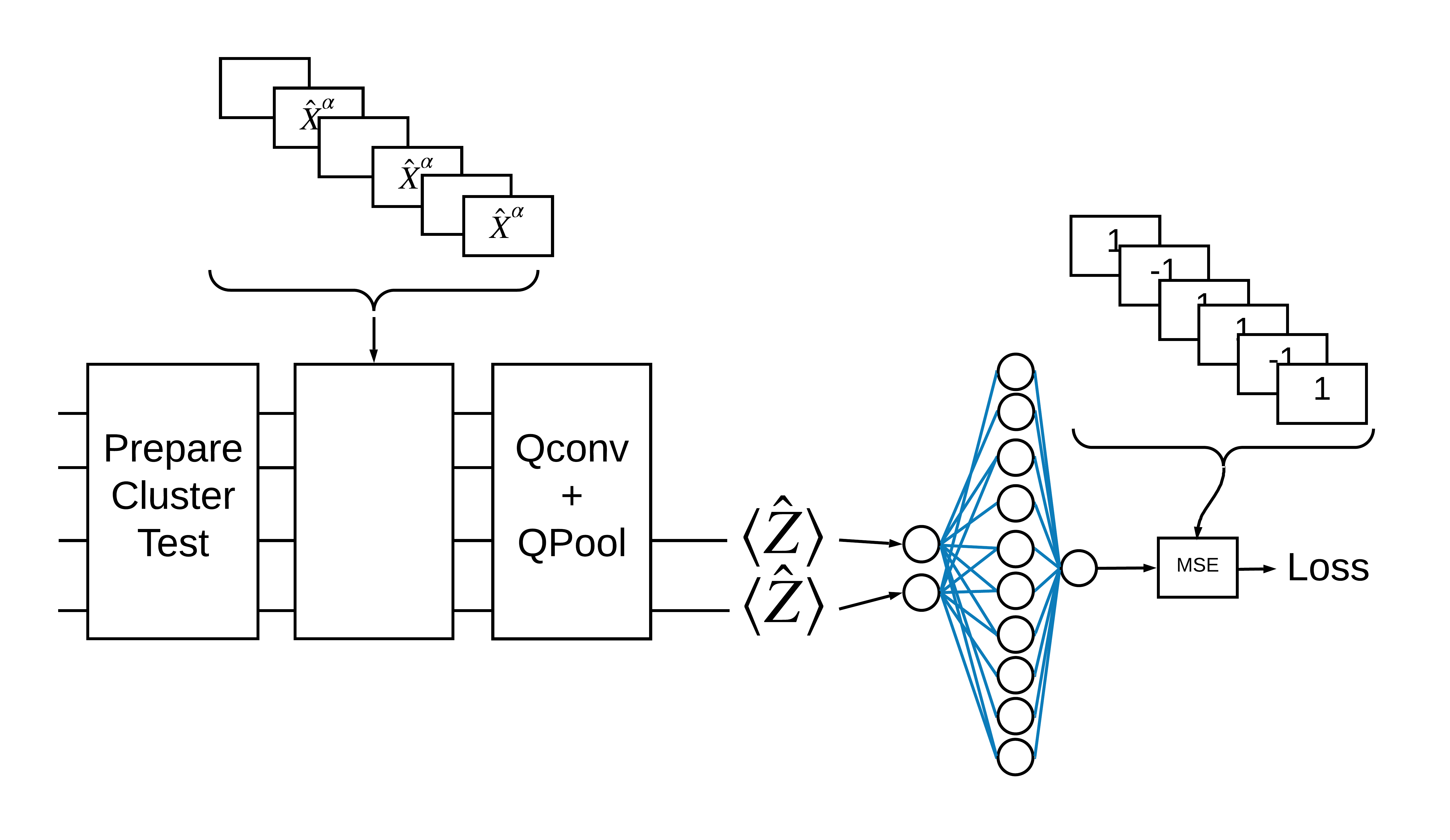
Un modo per risolvere questo problema con TensorFlow Quantum è implementare quanto segue:
- L'input del modello è un tensore del circuito, un circuito vuoto o una porta X su un particolare qubit che indica un'eccitazione.
- Il resto dei componenti quantistici del modello sono costruiti con i livelli
tfq.layers.AddCircuit. - Per l'inferenza viene utilizzato un livello
tfq.layers.PQC. Questo legge \(\langle \hat{Z} \rangle\) e lo confronta con un'etichetta di 1 per uno stato eccitato o -1 per uno stato non eccitato.
1.4 Dati
Prima di costruire il tuo modello, puoi generare i tuoi dati. In questo caso saranno eccitazioni allo stato del cluster (l'articolo originale utilizza un set di dati più complicato). Le eccitazioni sono rappresentate con porte cirq.rx Una rotazione sufficientemente grande è considerata un'eccitazione ed è etichettata 1 e una rotazione che non è abbastanza grande è etichettata -1 e considerata non un'eccitazione.
def generate_data(qubits):
    """Generate training and testing data."""
    n_rounds = 20  # Produces n_rounds * n_qubits datapoints.
    excitations = []
    labels = []
    for n in range(n_rounds):
        for bit in qubits:
            rng = np.random.uniform(-np.pi, np.pi)
            excitations.append(cirq.Circuit(cirq.rx(rng)(bit)))
            labels.append(1 if (-np.pi / 2) <= rng <= (np.pi / 2) else -1)

    split_ind = int(len(excitations) * 0.7)
    train_excitations = excitations[:split_ind]
    test_excitations = excitations[split_ind:]

    train_labels = labels[:split_ind]
    test_labels = labels[split_ind:]

    return tfq.convert_to_tensor(train_excitations), np.array(train_labels), \
        tfq.convert_to_tensor(test_excitations), np.array(test_labels)
Puoi vedere che, proprio come con il normale machine learning, crei un set di training e test da utilizzare per confrontare il modello. Puoi guardare rapidamente alcuni punti dati con:
sample_points, sample_labels, _, __ = generate_data(cirq.GridQubit.rect(1, 4))
print('Input:', tfq.from_tensor(sample_points)[0], 'Output:', sample_labels[0])
print('Input:', tfq.from_tensor(sample_points)[1], 'Output:', sample_labels[1])
Input: (0, 0): ───X^0.449─── Output: 1
Input: (0, 1): ───X^-0.74─── Output: -1
1.5 Definire i livelli
Ora definisci i livelli mostrati nella figura sopra in TensorFlow.
1.5.1 Stato del cluster
Il primo passaggio consiste nel definire lo stato del cluster utilizzando Cirq , un framework fornito da Google per la programmazione di circuiti quantistici. Poiché si tratta di una parte statica del modello, incorporarlo utilizzando la funzionalità tfq.layers.AddCircuit .
def cluster_state_circuit(bits):
    """Return a cluster state on the qubits in `bits`."""
    circuit = cirq.Circuit()
    circuit.append(cirq.H.on_each(bits))
    for this_bit, next_bit in zip(bits, bits[1:] + [bits[0]]):
        circuit.append(cirq.CZ(this_bit, next_bit))
    return circuit
Visualizza un circuito di stato del cluster per un rettangolo di cirq.GridQubit s:
SVGCircuit(cluster_state_circuit(cirq.GridQubit.rect(1, 4)))
findfont: Font family ['Arial'] not found. Falling back to DejaVu Sans.

1.5.2 Livelli QCNN
Definire gli strati che compongono il modello utilizzando la carta Cong e Lukin QCNN . Ci sono alcuni prerequisiti:
- Le matrici unitarie parametrizzate a uno e due qubit dall'articolo di Tucci .
- Un'operazione di pooling di due qubit parametrizzata generale.
def one_qubit_unitary(bit, symbols):
    """Make a Cirq circuit enacting a rotation of the bloch sphere about the X,
    Y and Z axis, that depends on the values in `symbols`.
    """
    return cirq.Circuit(
        cirq.X(bit)**symbols[0],
        cirq.Y(bit)**symbols[1],
        cirq.Z(bit)**symbols[2])


def two_qubit_unitary(bits, symbols):
    """Make a Cirq circuit that creates an arbitrary two qubit unitary."""
    circuit = cirq.Circuit()
    circuit += one_qubit_unitary(bits[0], symbols[0:3])
    circuit += one_qubit_unitary(bits[1], symbols[3:6])
    circuit += [cirq.ZZ(*bits)**symbols[6]]
    circuit += [cirq.YY(*bits)**symbols[7]]
    circuit += [cirq.XX(*bits)**symbols[8]]
    circuit += one_qubit_unitary(bits[0], symbols[9:12])
    circuit += one_qubit_unitary(bits[1], symbols[12:])
    return circuit


def two_qubit_pool(source_qubit, sink_qubit, symbols):
    """Make a Cirq circuit to do a parameterized 'pooling' operation, which
    attempts to reduce entanglement down from two qubits to just one."""
    pool_circuit = cirq.Circuit()
    sink_basis_selector = one_qubit_unitary(sink_qubit, symbols[0:3])
    source_basis_selector = one_qubit_unitary(source_qubit, symbols[3:6])
    pool_circuit.append(sink_basis_selector)
    pool_circuit.append(source_basis_selector)
    pool_circuit.append(cirq.CNOT(control=source_qubit, target=sink_qubit))
    pool_circuit.append(sink_basis_selector**-1)
    return pool_circuit
Per vedere cosa hai creato, stampa il circuito unitario di un qubit:
SVGCircuit(one_qubit_unitary(cirq.GridQubit(0, 0), sympy.symbols('x0:3')))

E il circuito unitario a due qubit:
SVGCircuit(two_qubit_unitary(cirq.GridQubit.rect(1, 2), sympy.symbols('x0:15')))

E il circuito di pooling a due qubit:
SVGCircuit(two_qubit_pool(*cirq.GridQubit.rect(1, 2), sympy.symbols('x0:6')))

1.5.2.1 Convoluzione quantistica
Come nel documento di Cong e Lukin , definisci la convoluzione quantistica 1D come l'applicazione di un parametro unitario di due qubit a ogni coppia di qubit adiacenti con un passo di uno.
def quantum_conv_circuit(bits, symbols):
    """Quantum Convolution Layer following the above diagram.
    Return a Cirq circuit with the cascade of `two_qubit_unitary` applied
    to all pairs of qubits in `bits` as in the diagram above.
    """
    circuit = cirq.Circuit()
    for first, second in zip(bits[0::2], bits[1::2]):
        circuit += two_qubit_unitary([first, second], symbols)
    for first, second in zip(bits[1::2], bits[2::2] + [bits[0]]):
        circuit += two_qubit_unitary([first, second], symbols)
    return circuit
Visualizza il circuito (molto orizzontale):
SVGCircuit(
    quantum_conv_circuit(cirq.GridQubit.rect(1, 8), sympy.symbols('x0:15')))

1.5.2.2 Raggruppamento quantistico
Un livello di pooling quantistico esegue il pool da \(N\) qubit a \(\frac{N}{2}\) qubit utilizzando il pool di due qubit definito sopra.
def quantum_pool_circuit(source_bits, sink_bits, symbols):
    """A layer that specifies a quantum pooling operation.
    A Quantum pool tries to learn to pool the relevant information from two
    qubits onto 1.
    """
    circuit = cirq.Circuit()
    for source, sink in zip(source_bits, sink_bits):
        circuit += two_qubit_pool(source, sink, symbols)
    return circuit
Esaminare un circuito di componenti di pooling:
test_bits = cirq.GridQubit.rect(1, 8)

SVGCircuit(
    quantum_pool_circuit(test_bits[:4], test_bits[4:], sympy.symbols('x0:6')))

1.6 Definizione del modello
Ora usa i livelli definiti per costruire una CNN puramente quantistica. Inizia con otto qubit, raggruppa fino a uno, quindi misura \(\langle \hat{Z} \rangle\).
def create_model_circuit(qubits):
"""Create sequence of alternating convolution and pooling operators
which gradually shrink over time."""
model_circuit = cirq.Circuit()
symbols = sympy.symbols('qconv0:63')
# Cirq uses sympy.Symbols to map learnable variables. TensorFlow Quantum
# scans incoming circuits and replaces these with TensorFlow variables.
model_circuit += quantum_conv_circuit(qubits, symbols[0:15])
model_circuit += quantum_pool_circuit(qubits[:4], qubits[4:],
symbols[15:21])
model_circuit += quantum_conv_circuit(qubits[4:], symbols[21:36])
model_circuit += quantum_pool_circuit(qubits[4:6], qubits[6:],
symbols[36:42])
model_circuit += quantum_conv_circuit(qubits[6:], symbols[42:57])
model_circuit += quantum_pool_circuit([qubits[6]], [qubits[7]],
symbols[57:63])
return model_circuit
# Create our qubits and readout operators in Cirq.
cluster_state_bits = cirq.GridQubit.rect(1, 8)
readout_operators = cirq.Z(cluster_state_bits[-1])
# Build a sequential model enacting the logic in 1.3 of this notebook.
# Here you are making the static cluster state prep as a part of the AddCircuit and the
# "quantum datapoints" are coming in the form of excitation
excitation_input = tf.keras.Input(shape=(), dtype=tf.dtypes.string)
cluster_state = tfq.layers.AddCircuit()(
excitation_input, prepend=cluster_state_circuit(cluster_state_bits))
quantum_model = tfq.layers.PQC(create_model_circuit(cluster_state_bits),
readout_operators)(cluster_state)
qcnn_model = tf.keras.Model(inputs=[excitation_input], outputs=[quantum_model])
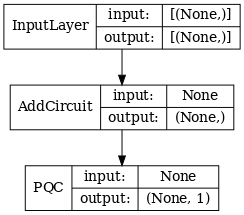
# Show the keras plot of the model
tf.keras.utils.plot_model(qcnn_model,
show_shapes=True,
show_layer_names=False,
dpi=70)
1.7 Addestrare il modello
Addestrare il modello sull'intero batch per semplificare questo esempio.
# Generate some training data.
train_excitations, train_labels, test_excitations, test_labels = generate_data(
    cluster_state_bits)


# Custom accuracy metric.
@tf.function
def custom_accuracy(y_true, y_pred):
    y_true = tf.squeeze(y_true)
    y_pred = tf.map_fn(lambda x: 1.0 if x >= 0 else -1.0, y_pred)
    return tf.keras.backend.mean(tf.keras.backend.equal(y_true, y_pred))


qcnn_model.compile(optimizer=tf.keras.optimizers.Adam(learning_rate=0.02),
                   loss=tf.losses.mse,
                   metrics=[custom_accuracy])

history = qcnn_model.fit(x=train_excitations,
                         y=train_labels,
                         batch_size=16,
                         epochs=25,
                         verbose=1,
                         validation_data=(test_excitations, test_labels))
Epoch 1/25
7/7 [==============================] - 2s 176ms/step - loss: 0.8961 - custom_accuracy: 0.7143 - val_loss: 0.8012 - val_custom_accuracy: 0.7500
Epoch 2/25
7/7 [==============================] - 1s 140ms/step - loss: 0.7736 - custom_accuracy: 0.7946 - val_loss: 0.7355 - val_custom_accuracy: 0.8542
Epoch 3/25
7/7 [==============================] - 1s 138ms/step - loss: 0.7319 - custom_accuracy: 0.8393 - val_loss: 0.7045 - val_custom_accuracy: 0.8125
Epoch 4/25
7/7 [==============================] - 1s 137ms/step - loss: 0.6976 - custom_accuracy: 0.8482 - val_loss: 0.6829 - val_custom_accuracy: 0.8333
Epoch 5/25
7/7 [==============================] - 1s 143ms/step - loss: 0.6696 - custom_accuracy: 0.8750 - val_loss: 0.6749 - val_custom_accuracy: 0.7917
Epoch 6/25
7/7 [==============================] - 1s 137ms/step - loss: 0.6631 - custom_accuracy: 0.8750 - val_loss: 0.6718 - val_custom_accuracy: 0.7917
Epoch 7/25
7/7 [==============================] - 1s 135ms/step - loss: 0.6536 - custom_accuracy: 0.8929 - val_loss: 0.6638 - val_custom_accuracy: 0.8750
Epoch 8/25
7/7 [==============================] - 1s 141ms/step - loss: 0.6376 - custom_accuracy: 0.8750 - val_loss: 0.6311 - val_custom_accuracy: 0.8542
Epoch 9/25
7/7 [==============================] - 1s 137ms/step - loss: 0.6208 - custom_accuracy: 0.8750 - val_loss: 0.5995 - val_custom_accuracy: 0.8542
Epoch 10/25
7/7 [==============================] - 1s 134ms/step - loss: 0.5887 - custom_accuracy: 0.8661 - val_loss: 0.5655 - val_custom_accuracy: 0.8333
Epoch 11/25
7/7 [==============================] - 1s 144ms/step - loss: 0.5796 - custom_accuracy: 0.8482 - val_loss: 0.5681 - val_custom_accuracy: 0.8333
Epoch 12/25
7/7 [==============================] - 1s 143ms/step - loss: 0.5630 - custom_accuracy: 0.7946 - val_loss: 0.5179 - val_custom_accuracy: 0.8333
Epoch 13/25
7/7 [==============================] - 1s 137ms/step - loss: 0.5405 - custom_accuracy: 0.8304 - val_loss: 0.5003 - val_custom_accuracy: 0.8333
Epoch 14/25
7/7 [==============================] - 1s 138ms/step - loss: 0.5259 - custom_accuracy: 0.8036 - val_loss: 0.4787 - val_custom_accuracy: 0.8333
Epoch 15/25
7/7 [==============================] - 1s 137ms/step - loss: 0.5077 - custom_accuracy: 0.8482 - val_loss: 0.4741 - val_custom_accuracy: 0.8125
Epoch 16/25
7/7 [==============================] - 1s 136ms/step - loss: 0.5082 - custom_accuracy: 0.8214 - val_loss: 0.4739 - val_custom_accuracy: 0.8125
Epoch 17/25
7/7 [==============================] - 1s 137ms/step - loss: 0.5138 - custom_accuracy: 0.8214 - val_loss: 0.4859 - val_custom_accuracy: 0.8750
Epoch 18/25
7/7 [==============================] - 1s 133ms/step - loss: 0.5073 - custom_accuracy: 0.8304 - val_loss: 0.4879 - val_custom_accuracy: 0.8333
Epoch 19/25
7/7 [==============================] - 1s 138ms/step - loss: 0.5084 - custom_accuracy: 0.8304 - val_loss: 0.4745 - val_custom_accuracy: 0.8542
Epoch 20/25
7/7 [==============================] - 1s 139ms/step - loss: 0.5057 - custom_accuracy: 0.8571 - val_loss: 0.4702 - val_custom_accuracy: 0.8333
Epoch 21/25
7/7 [==============================] - 1s 135ms/step - loss: 0.4939 - custom_accuracy: 0.8304 - val_loss: 0.4734 - val_custom_accuracy: 0.8750
Epoch 22/25
7/7 [==============================] - 1s 138ms/step - loss: 0.4942 - custom_accuracy: 0.8750 - val_loss: 0.4725 - val_custom_accuracy: 0.8750
Epoch 23/25
7/7 [==============================] - 1s 140ms/step - loss: 0.4982 - custom_accuracy: 0.9107 - val_loss: 0.4695 - val_custom_accuracy: 0.8958
Epoch 24/25
7/7 [==============================] - 1s 135ms/step - loss: 0.4936 - custom_accuracy: 0.8661 - val_loss: 0.4731 - val_custom_accuracy: 0.8750
Epoch 25/25
7/7 [==============================] - 1s 136ms/step - loss: 0.4866 - custom_accuracy: 0.8571 - val_loss: 0.4631 - val_custom_accuracy: 0.8958
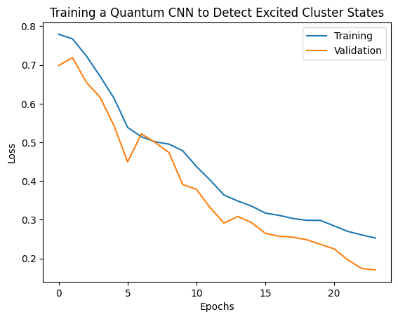
plt.plot(history.history['loss'][1:], label='Training')
plt.plot(history.history['val_loss'][1:], label='Validation')
plt.title('Training a Quantum CNN to Detect Excited Cluster States')
plt.xlabel('Epochs')
plt.ylabel('Loss')
plt.legend()
plt.show()
2. Modelli ibridi
Non è necessario passare da otto qubit a un qubit usando la convoluzione quantistica: avresti potuto eseguire uno o due cicli di convoluzione quantistica e inserire i risultati in una rete neurale classica. Questa sezione esplora i modelli ibridi quantistici classici.
2.1 Modello ibrido con un unico filtro quantistico
Applicare uno strato di convoluzione quantistica, leggendo \(\langle \hat{Z}_n \rangle\) su tutti i bit, seguito da una rete neurale densamente connessa.
2.1.1 Definizione del modello
# 1-local operators to read out
readouts = [cirq.Z(bit) for bit in cluster_state_bits[4:]]
def multi_readout_model_circuit(qubits):
"""Make a model circuit with less quantum pool and conv operations."""
model_circuit = cirq.Circuit()
symbols = sympy.symbols('qconv0:21')
model_circuit += quantum_conv_circuit(qubits, symbols[0:15])
model_circuit += quantum_pool_circuit(qubits[:4], qubits[4:],
symbols[15:21])
return model_circuit
# Build a model enacting the logic in 2.1 of this notebook.
excitation_input_dual = tf.keras.Input(shape=(), dtype=tf.dtypes.string)
cluster_state_dual = tfq.layers.AddCircuit()(
excitation_input_dual, prepend=cluster_state_circuit(cluster_state_bits))
quantum_model_dual = tfq.layers.PQC(
multi_readout_model_circuit(cluster_state_bits),
readouts)(cluster_state_dual)
d1_dual = tf.keras.layers.Dense(8)(quantum_model_dual)
d2_dual = tf.keras.layers.Dense(1)(d1_dual)
hybrid_model = tf.keras.Model(inputs=[excitation_input_dual], outputs=[d2_dual])
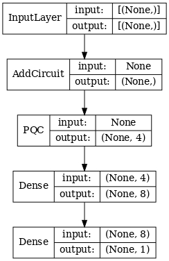
# Display the model architecture
tf.keras.utils.plot_model(hybrid_model,
show_shapes=True,
show_layer_names=False,
dpi=70)
2.1.2 Addestrare il modello
hybrid_model.compile(optimizer=tf.keras.optimizers.Adam(learning_rate=0.02),
                     loss=tf.losses.mse,
                     metrics=[custom_accuracy])

hybrid_history = hybrid_model.fit(x=train_excitations,
                                  y=train_labels,
                                  batch_size=16,
                                  epochs=25,
                                  verbose=1,
                                  validation_data=(test_excitations,
                                                   test_labels))
Epoch 1/25
7/7 [==============================] - 1s 113ms/step - loss: 0.9848 - custom_accuracy: 0.5179 - val_loss: 0.9635 - val_custom_accuracy: 0.5417
Epoch 2/25
7/7 [==============================] - 1s 86ms/step - loss: 0.8095 - custom_accuracy: 0.6339 - val_loss: 0.6800 - val_custom_accuracy: 0.7083
Epoch 3/25
7/7 [==============================] - 1s 85ms/step - loss: 0.4045 - custom_accuracy: 0.9375 - val_loss: 0.3342 - val_custom_accuracy: 0.8750
Epoch 4/25
7/7 [==============================] - 1s 86ms/step - loss: 0.2308 - custom_accuracy: 0.9643 - val_loss: 0.2027 - val_custom_accuracy: 0.9792
Epoch 5/25
7/7 [==============================] - 1s 84ms/step - loss: 0.2232 - custom_accuracy: 0.9554 - val_loss: 0.1761 - val_custom_accuracy: 1.0000
Epoch 6/25
7/7 [==============================] - 1s 84ms/step - loss: 0.1760 - custom_accuracy: 0.9821 - val_loss: 0.2541 - val_custom_accuracy: 0.9167
Epoch 7/25
7/7 [==============================] - 1s 85ms/step - loss: 0.1919 - custom_accuracy: 0.9643 - val_loss: 0.1967 - val_custom_accuracy: 0.9792
Epoch 8/25
7/7 [==============================] - 1s 83ms/step - loss: 0.1892 - custom_accuracy: 0.9554 - val_loss: 0.1870 - val_custom_accuracy: 0.9792
Epoch 9/25
7/7 [==============================] - 1s 84ms/step - loss: 0.1777 - custom_accuracy: 0.9911 - val_loss: 0.2208 - val_custom_accuracy: 0.9583
Epoch 10/25
7/7 [==============================] - 1s 83ms/step - loss: 0.1728 - custom_accuracy: 0.9732 - val_loss: 0.2147 - val_custom_accuracy: 0.9583
Epoch 11/25
7/7 [==============================] - 1s 85ms/step - loss: 0.1704 - custom_accuracy: 0.9732 - val_loss: 0.1810 - val_custom_accuracy: 0.9792
Epoch 12/25
7/7 [==============================] - 1s 85ms/step - loss: 0.1739 - custom_accuracy: 0.9732 - val_loss: 0.2038 - val_custom_accuracy: 0.9792
Epoch 13/25
7/7 [==============================] - 1s 81ms/step - loss: 0.1705 - custom_accuracy: 0.9732 - val_loss: 0.1855 - val_custom_accuracy: 0.9792
Epoch 14/25
7/7 [==============================] - 1s 84ms/step - loss: 0.1788 - custom_accuracy: 0.9643 - val_loss: 0.2152 - val_custom_accuracy: 0.9583
Epoch 15/25
7/7 [==============================] - 1s 84ms/step - loss: 0.1760 - custom_accuracy: 0.9732 - val_loss: 0.1994 - val_custom_accuracy: 1.0000
Epoch 16/25
7/7 [==============================] - 1s 83ms/step - loss: 0.1737 - custom_accuracy: 0.9732 - val_loss: 0.2035 - val_custom_accuracy: 0.9792
Epoch 17/25
7/7 [==============================] - 1s 82ms/step - loss: 0.1749 - custom_accuracy: 0.9911 - val_loss: 0.1983 - val_custom_accuracy: 0.9583
Epoch 18/25
7/7 [==============================] - 1s 83ms/step - loss: 0.1875 - custom_accuracy: 0.9732 - val_loss: 0.1916 - val_custom_accuracy: 0.9583
Epoch 19/25
7/7 [==============================] - 1s 82ms/step - loss: 0.1605 - custom_accuracy: 0.9732 - val_loss: 0.1782 - val_custom_accuracy: 0.9792
Epoch 20/25
7/7 [==============================] - 1s 84ms/step - loss: 0.1668 - custom_accuracy: 0.9911 - val_loss: 0.2276 - val_custom_accuracy: 0.9583
Epoch 21/25
7/7 [==============================] - 1s 84ms/step - loss: 0.1700 - custom_accuracy: 0.9911 - val_loss: 0.2080 - val_custom_accuracy: 0.9583
Epoch 22/25
7/7 [==============================] - 1s 83ms/step - loss: 0.1621 - custom_accuracy: 0.9732 - val_loss: 0.1851 - val_custom_accuracy: 0.9375
Epoch 23/25
7/7 [==============================] - 1s 84ms/step - loss: 0.1695 - custom_accuracy: 0.9911 - val_loss: 0.1882 - val_custom_accuracy: 0.9792
Epoch 24/25
7/7 [==============================] - 1s 82ms/step - loss: 0.1583 - custom_accuracy: 0.9911 - val_loss: 0.2017 - val_custom_accuracy: 0.9583
Epoch 25/25
7/7 [==============================] - 1s 83ms/step - loss: 0.1557 - custom_accuracy: 0.9911 - val_loss: 0.1907 - val_custom_accuracy: 0.9792
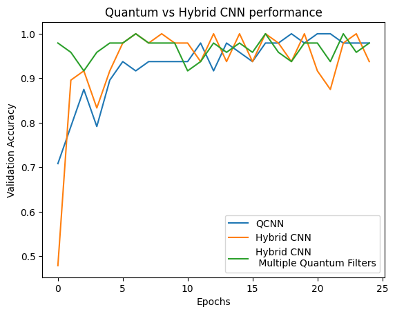
plt.plot(history.history['val_custom_accuracy'], label='QCNN')
plt.plot(hybrid_history.history['val_custom_accuracy'], label='Hybrid CNN')
plt.title('Quantum vs Hybrid CNN performance')
plt.xlabel('Epochs')
plt.legend()
plt.ylabel('Validation Accuracy')
plt.show()
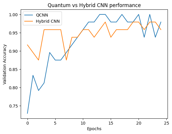
Come puoi vedere, con un'assistenza classica molto modesta, il modello ibrido convergerà solitamente più velocemente rispetto alla versione puramente quantistica.
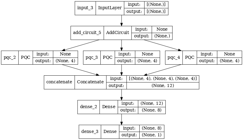
2.2 Convoluzione ibrida con più filtri quantistici
Ora proviamo un'architettura che utilizza più convoluzioni quantistiche e una rete neurale classica per combinarle.
2.2.1 Definizione del modello
excitation_input_multi = tf.keras.Input(shape=(), dtype=tf.dtypes.string)

cluster_state_multi = tfq.layers.AddCircuit()(
    excitation_input_multi, prepend=cluster_state_circuit(cluster_state_bits))

# apply 3 different filters and measure expectation values

quantum_model_multi1 = tfq.layers.PQC(
    multi_readout_model_circuit(cluster_state_bits),
    readouts)(cluster_state_multi)

quantum_model_multi2 = tfq.layers.PQC(
    multi_readout_model_circuit(cluster_state_bits),
    readouts)(cluster_state_multi)

quantum_model_multi3 = tfq.layers.PQC(
    multi_readout_model_circuit(cluster_state_bits),
    readouts)(cluster_state_multi)

# concatenate outputs and feed into a small classical NN
concat_out = tf.keras.layers.concatenate(
    [quantum_model_multi1, quantum_model_multi2, quantum_model_multi3])

dense_1 = tf.keras.layers.Dense(8)(concat_out)

dense_2 = tf.keras.layers.Dense(1)(dense_1)

multi_qconv_model = tf.keras.Model(inputs=[excitation_input_multi],
                                   outputs=[dense_2])

# Display the model architecture
tf.keras.utils.plot_model(multi_qconv_model,
                          show_shapes=True,
                          show_layer_names=True,
                          dpi=70)
2.2.2 Addestrare il modello
multi_qconv_model.compile(
    optimizer=tf.keras.optimizers.Adam(learning_rate=0.02),
    loss=tf.losses.mse,
    metrics=[custom_accuracy])

multi_qconv_history = multi_qconv_model.fit(x=train_excitations,
                                            y=train_labels,
                                            batch_size=16,
                                            epochs=25,
                                            verbose=1,
                                            validation_data=(test_excitations,
                                                             test_labels))
Epoch 1/25
7/7 [==============================] - 2s 143ms/step - loss: 0.9425 - custom_accuracy: 0.6429 - val_loss: 0.8120 - val_custom_accuracy: 0.7083
Epoch 2/25
7/7 [==============================] - 1s 109ms/step - loss: 0.5778 - custom_accuracy: 0.7946 - val_loss: 0.5920 - val_custom_accuracy: 0.7500
Epoch 3/25
7/7 [==============================] - 1s 103ms/step - loss: 0.4954 - custom_accuracy: 0.9018 - val_loss: 0.4568 - val_custom_accuracy: 0.7708
Epoch 4/25
7/7 [==============================] - 1s 95ms/step - loss: 0.2855 - custom_accuracy: 0.9196 - val_loss: 0.2792 - val_custom_accuracy: 0.9375
Epoch 5/25
7/7 [==============================] - 1s 93ms/step - loss: 0.1902 - custom_accuracy: 0.9821 - val_loss: 0.2212 - val_custom_accuracy: 0.9375
Epoch 6/25
7/7 [==============================] - 1s 94ms/step - loss: 0.1685 - custom_accuracy: 0.9821 - val_loss: 0.2341 - val_custom_accuracy: 0.9583
Epoch 7/25
7/7 [==============================] - 1s 104ms/step - loss: 0.1671 - custom_accuracy: 0.9911 - val_loss: 0.2062 - val_custom_accuracy: 0.9792
Epoch 8/25
7/7 [==============================] - 1s 97ms/step - loss: 0.1511 - custom_accuracy: 0.9821 - val_loss: 0.2096 - val_custom_accuracy: 0.9792
Epoch 9/25
7/7 [==============================] - 1s 96ms/step - loss: 0.1432 - custom_accuracy: 0.9911 - val_loss: 0.2330 - val_custom_accuracy: 0.9375
Epoch 10/25
7/7 [==============================] - 1s 92ms/step - loss: 0.1668 - custom_accuracy: 0.9821 - val_loss: 0.2344 - val_custom_accuracy: 0.9583
Epoch 11/25
7/7 [==============================] - 1s 106ms/step - loss: 0.1893 - custom_accuracy: 0.9732 - val_loss: 0.2148 - val_custom_accuracy: 0.9583
Epoch 12/25
7/7 [==============================] - 1s 104ms/step - loss: 0.1857 - custom_accuracy: 0.9732 - val_loss: 0.2739 - val_custom_accuracy: 0.9583
Epoch 13/25
7/7 [==============================] - 1s 106ms/step - loss: 0.1748 - custom_accuracy: 0.9732 - val_loss: 0.2366 - val_custom_accuracy: 0.9583
Epoch 14/25
7/7 [==============================] - 1s 103ms/step - loss: 0.1515 - custom_accuracy: 0.9821 - val_loss: 0.2012 - val_custom_accuracy: 0.9583
Epoch 15/25
7/7 [==============================] - 1s 100ms/step - loss: 0.1552 - custom_accuracy: 0.9911 - val_loss: 0.2404 - val_custom_accuracy: 0.9375
Epoch 16/25
7/7 [==============================] - 1s 97ms/step - loss: 0.1572 - custom_accuracy: 0.9911 - val_loss: 0.2779 - val_custom_accuracy: 0.9375
Epoch 17/25
7/7 [==============================] - 1s 100ms/step - loss: 0.1546 - custom_accuracy: 0.9821 - val_loss: 0.2104 - val_custom_accuracy: 0.9583
Epoch 18/25
7/7 [==============================] - 1s 102ms/step - loss: 0.1418 - custom_accuracy: 0.9911 - val_loss: 0.2647 - val_custom_accuracy: 0.9583
Epoch 19/25
7/7 [==============================] - 1s 98ms/step - loss: 0.1590 - custom_accuracy: 0.9732 - val_loss: 0.2154 - val_custom_accuracy: 0.9583
Epoch 20/25
7/7 [==============================] - 1s 104ms/step - loss: 0.1363 - custom_accuracy: 1.0000 - val_loss: 0.2470 - val_custom_accuracy: 0.9375
Epoch 21/25
7/7 [==============================] - 1s 100ms/step - loss: 0.1442 - custom_accuracy: 0.9821 - val_loss: 0.2383 - val_custom_accuracy: 0.9375
Epoch 22/25
7/7 [==============================] - 1s 99ms/step - loss: 0.1415 - custom_accuracy: 0.9911 - val_loss: 0.2324 - val_custom_accuracy: 0.9583
Epoch 23/25
7/7 [==============================] - 1s 97ms/step - loss: 0.1424 - custom_accuracy: 0.9821 - val_loss: 0.2188 - val_custom_accuracy: 0.9583
Epoch 24/25
7/7 [==============================] - 1s 100ms/step - loss: 0.1417 - custom_accuracy: 0.9821 - val_loss: 0.2340 - val_custom_accuracy: 0.9375
Epoch 25/25
7/7 [==============================] - 1s 103ms/step - loss: 0.1471 - custom_accuracy: 0.9732 - val_loss: 0.2252 - val_custom_accuracy: 0.9583
plt.plot(history.history['val_custom_accuracy'][:25], label='QCNN')
plt.plot(hybrid_history.history['val_custom_accuracy'][:25], label='Hybrid CNN')
plt.plot(multi_qconv_history.history['val_custom_accuracy'][:25],
         label='Hybrid CNN \n Multiple Quantum Filters')
plt.title('Quantum vs Hybrid CNN performance')
plt.xlabel('Epochs')
plt.legend()
plt.ylabel('Validation Accuracy')
plt.show()