
| | |  GitHub에서 소스 보기 GitHub에서 소스 보기 |
이 튜토리얼은 Transformer 모델 을 학습시켜 포르투갈어를 영어 데이터 세트 로 번역합니다. 이것은 텍스트 생성 및 주의 에 대한 지식을 가정한 고급 예제입니다.
Transformer 모델의 핵심 아이디어는 self-attention (입력 시퀀스의 표현을 계산하기 위해 입력 시퀀스의 다른 위치에 주의를 기울이는 기능)입니다. Transformer는 self-attention 레이어의 스택을 생성하고 아래의 Scaled dot product Attention 및 Multi-head Attention 섹션에서 설명됩니다.
변환기 모델은 RNN 또는 CNN 대신 자체 주의 계층 스택을 사용하여 가변 크기 입력을 처리합니다. 이 일반 아키텍처에는 다음과 같은 여러 장점이 있습니다.
- 데이터 전반에 걸친 시간적/공간적 관계에 대해 가정하지 않습니다. 이는 개체 집합(예: StarCraft 단위 )을 처리하는 데 이상적입니다.
- 레이어 출력은 RNN과 같은 시리즈 대신 병렬로 계산할 수 있습니다.
- 멀리 있는 항목은 많은 RNN 단계 또는 컨볼루션 레이어를 거치지 않고 서로의 출력에 영향을 줄 수 있습니다(예: Scene Memory Transformer 참조).
- 장거리 종속성을 학습할 수 있습니다. 이것은 많은 시퀀스 작업의 도전과제입니다.
이 아키텍처의 단점은 다음과 같습니다.
- 시계열의 경우 시간 단계에 대한 출력은 입력 및 현재 숨겨진 상태 대신 전체 기록 에서 계산됩니다. 이것은 덜 효율적일 수 있습니다.
- 입력에 텍스트와 같은 시간적/공간적 관계 가 있는 경우 일부 위치 인코딩을 추가해야 합니다. 그렇지 않으면 모델이 단어 모음을 효과적으로 볼 수 있습니다.
이 노트북에서 모델을 훈련시킨 후, 포르투갈어 문장을 입력하고 영어 번역을 반환할 수 있습니다.
설정
pip install tensorflow_datasetspip install -U tensorflow-text
import collections
import logging
import os
import pathlib
import re
import string
import sys
import time

import numpy as np
import matplotlib.pyplot as plt

import tensorflow_datasets as tfds
import tensorflow_text as text
import tensorflow as tf
logging.getLogger('tensorflow').setLevel(logging.ERROR) # suppress warnings
데이터세트 다운로드
TensorFlow 데이터세트 를 사용하여 TED Talks Open Translation Project 에서 포르투갈어-영어 번역 데이터 세트를 로드하세요.
이 데이터 세트에는 약 50000개의 교육 예제, 1100개의 검증 예제 및 2000개의 테스트 예제가 포함되어 있습니다.
examples, metadata = tfds.load('ted_hrlr_translate/pt_to_en', with_info=True,
                               as_supervised=True)
train_examples, val_examples = examples['train'], examples['validation']
TensorFlow 데이터 세트에서 반환된 tf.data.Dataset 객체는 텍스트 예제 쌍을 생성합니다.
for pt_examples, en_examples in train_examples.batch(3).take(1):
  for pt in pt_examples.numpy():
    print(pt.decode('utf-8'))

  print()

  for en in en_examples.numpy():
    print(en.decode('utf-8'))
e quando melhoramos a procura , tiramos a única vantagem da impressão , que é a serendipidade .
mas e se estes fatores fossem ativos ?
mas eles não tinham a curiosidade de me testar .

and when you improve searchability , you actually take away the one advantage of print , which is serendipity .
but what if it were active ?
but they did n't test for curiosity .
텍스트 토큰화 및 해독
텍스트에서 직접 모델을 훈련할 수는 없습니다. 먼저 텍스트를 숫자 표현으로 변환해야 합니다. 일반적으로 텍스트를 포함에 대한 인덱스로 사용되는 토큰 ID 시퀀스로 변환합니다.
인기 있는 구현 중 하나는 Subword 토크나이저 자습서 에서 이 데이터세트에 최적화된 하위 단어 토크나이저( text.BertTokenizer )를 빌드하고 stored_model 로 내보냅니다.
saved_model 을 다운로드하고 압축을 풀고 가져옵니다.
model_name = "ted_hrlr_translate_pt_en_converter"
tf.keras.utils.get_file(
    f"{model_name}.zip",
    f"https://storage.googleapis.com/download.tensorflow.org/models/{model_name}.zip",
    cache_dir='.', cache_subdir='', extract=True
)
Downloading data from https://storage.googleapis.com/download.tensorflow.org/models/ted_hrlr_translate_pt_en_converter.zip
188416/184801 [==============================] - 0s 0us/step
196608/184801 [===============================] - 0s 0us/step
'./ted_hrlr_translate_pt_en_converter.zip'
tokenizers = tf.saved_model.load(model_name)
tf.saved_model 에는 두 개의 텍스트 토크나이저가 포함되어 있습니다. 하나는 영어용이고 다른 하나는 포르투갈어용입니다. 둘 다 동일한 방법을 사용합니다.
[item for item in dir(tokenizers.en) if not item.startswith('_')]
['detokenize',
 'get_reserved_tokens',
 'get_vocab_path',
 'get_vocab_size',
 'lookup',
 'tokenize',
 'tokenizer',
 'vocab']
tokenize 메서드는 문자열 배치를 토큰 ID의 패딩 배치로 변환합니다. 이 방법은 구두점, 소문자를 분할하고 토큰화하기 전에 입력을 유니코드 정규화합니다. 입력 데이터가 이미 표준화되어 있기 때문에 해당 표준화는 여기에 표시되지 않습니다.
for en in en_examples.numpy():
  print(en.decode('utf-8'))
and when you improve searchability , you actually take away the one advantage of print , which is serendipity .
but what if it were active ?
but they did n't test for curiosity .
encoded = tokenizers.en.tokenize(en_examples)

for row in encoded.to_list():
  print(row)
[2, 72, 117, 79, 1259, 1491, 2362, 13, 79, 150, 184, 311, 71, 103, 2308, 74, 2679, 13, 148, 80, 55, 4840, 1434, 2423, 540, 15, 3]
[2, 87, 90, 107, 76, 129, 1852, 30, 3]
[2, 87, 83, 149, 50, 9, 56, 664, 85, 2512, 15, 3]
detokenize 메서드는 이러한 토큰 ID를 사람이 읽을 수 있는 텍스트로 다시 변환하려고 시도합니다.
round_trip = tokenizers.en.detokenize(encoded)
for line in round_trip.numpy():
  print(line.decode('utf-8'))
and when you improve searchability , you actually take away the one advantage of print , which is serendipity .
but what if it were active ?
but they did n ' t test for curiosity .
하위 수준 lookup 방법은 토큰 ID에서 토큰 텍스트로 변환합니다.
tokens = tokenizers.en.lookup(encoded)
tokens
<tf.RaggedTensor [[b'[START]', b'and', b'when', b'you', b'improve', b'search', b'##ability',
  b',', b'you', b'actually', b'take', b'away', b'the', b'one', b'advantage',
  b'of', b'print', b',', b'which', b'is', b's', b'##ere', b'##nd', b'##ip',
  b'##ity', b'.', b'[END]']                                                 ,
 [b'[START]', b'but', b'what', b'if', b'it', b'were', b'active', b'?',
  b'[END]']                                                           ,
 [b'[START]', b'but', b'they', b'did', b'n', b"'", b't', b'test', b'for',
  b'curiosity', b'.', b'[END]']                                          ]>
여기에서 토크나이저의 "하위 단어" 측면을 볼 수 있습니다. "searchability"라는 단어는 "search ##ability"로, "serendipity"라는 단어는 "s ##ere ##nd ##ip ##ity"로 분해됩니다.
입력 파이프라인 설정
훈련에 적합한 입력 파이프라인을 구축하기 위해 데이터 세트에 몇 가지 변환을 적용합니다.
이 함수는 원시 텍스트 배치를 인코딩하는 데 사용됩니다.
def tokenize_pairs(pt, en):
    pt = tokenizers.pt.tokenize(pt)
    # Convert from ragged to dense, padding with zeros.
    pt = pt.to_tensor()

    en = tokenizers.en.tokenize(en)
    # Convert from ragged to dense, padding with zeros.
    en = en.to_tensor()
    return pt, en
다음은 데이터를 처리, 셔플 및 일괄 처리하는 간단한 입력 파이프라인입니다.
BUFFER_SIZE = 20000
BATCH_SIZE = 64
def make_batches(ds):
  return (
      ds
      .cache()
      .shuffle(BUFFER_SIZE)
      .batch(BATCH_SIZE)
      .map(tokenize_pairs, num_parallel_calls=tf.data.AUTOTUNE)
      .prefetch(tf.data.AUTOTUNE))


train_batches = make_batches(train_examples)
val_batches = make_batches(val_examples)
위치 인코딩
어텐션 레이어는 입력을 순차적인 순서가 없는 벡터 세트로 봅니다. 이 모델에는 순환 또는 컨볼루션 레이어도 포함되어 있지 않습니다. 이 때문에 "위치 인코딩"이 추가되어 모델에 문장에서 토큰의 상대적 위치에 대한 정보를 제공합니다.
위치 인코딩 벡터가 임베딩 벡터에 추가됩니다. 임베딩은 비슷한 의미를 가진 토큰이 서로 더 가까워지는 d차원 공간의 토큰을 나타냅니다. 그러나 임베딩은 문장에서 토큰의 상대적 위치를 인코딩하지 않습니다. 따라서 위치 인코딩을 추가한 후 토큰은 d차원 공간 에서 의미의 유사성과 문장에서의 위치에 따라 서로 더 가까워집니다.
위치 인코딩을 계산하는 공식은 다음과 같습니다.
\[\Large{PE_{(pos, 2i)} = \sin(pos / 10000^{2i / d_{model} })} \]
\[\Large{PE_{(pos, 2i+1)} = \cos(pos / 10000^{2i / d_{model} })} \]
def get_angles(pos, i, d_model):
  angle_rates = 1 / np.power(10000, (2 * (i//2)) / np.float32(d_model))
  return pos * angle_rates
def positional_encoding(position, d_model):
  angle_rads = get_angles(np.arange(position)[:, np.newaxis],
                          np.arange(d_model)[np.newaxis, :],
                          d_model)

  # apply sin to even indices in the array; 2i
  angle_rads[:, 0::2] = np.sin(angle_rads[:, 0::2])

  # apply cos to odd indices in the array; 2i+1
  angle_rads[:, 1::2] = np.cos(angle_rads[:, 1::2])

  pos_encoding = angle_rads[np.newaxis, ...]

  return tf.cast(pos_encoding, dtype=tf.float32)
n, d = 2048, 512
pos_encoding = positional_encoding(n, d)
print(pos_encoding.shape)
pos_encoding = pos_encoding[0]

# Juggle the dimensions for the plot
pos_encoding = tf.reshape(pos_encoding, (n, d//2, 2))
pos_encoding = tf.transpose(pos_encoding, (2, 1, 0))
pos_encoding = tf.reshape(pos_encoding, (d, n))

plt.pcolormesh(pos_encoding, cmap='RdBu')
plt.ylabel('Depth')
plt.xlabel('Position')
plt.colorbar()
plt.show()
(1, 2048, 512)

마스킹
시퀀스 배치에서 모든 패드 토큰을 마스킹합니다. 모델이 패딩을 입력으로 취급하지 않도록 합니다. 마스크는 패드 값 0 이 있는 위치를 나타냅니다. 해당 위치에서 1 을 출력하고 그렇지 않으면 0 을 출력합니다.
def create_padding_mask(seq):
  seq = tf.cast(tf.math.equal(seq, 0), tf.float32)

  # add extra dimensions to add the padding
  # to the attention logits.
  return seq[:, tf.newaxis, tf.newaxis, :]  # (batch_size, 1, 1, seq_len)
x = tf.constant([[7, 6, 0, 0, 1], [1, 2, 3, 0, 0], [0, 0, 0, 4, 5]])
create_padding_mask(x)
<tf.Tensor: shape=(3, 1, 1, 5), dtype=float32, numpy=
array([[[[0., 0., 1., 1., 0.]]],


       [[[0., 0., 0., 1., 1.]]],


       [[[1., 1., 1., 0., 0.]]]], dtype=float32)>
미리보기 마스크는 시퀀스에서 미래 토큰을 마스킹하는 데 사용됩니다. 즉, 마스크는 사용해서는 안 되는 항목을 나타냅니다.
즉, 세 번째 토큰을 예측하기 위해 첫 번째와 두 번째 토큰만 사용됩니다. 네 번째 토큰을 예측하는 것과 유사하게 첫 번째, 두 번째 및 세 번째 토큰만 사용됩니다.
def create_look_ahead_mask(size):
  mask = 1 - tf.linalg.band_part(tf.ones((size, size)), -1, 0)
  return mask  # (seq_len, seq_len)
x = tf.random.uniform((1, 3))
temp = create_look_ahead_mask(x.shape[1])
temp
<tf.Tensor: shape=(3, 3), dtype=float32, numpy=
array([[0., 1., 1.],
       [0., 0., 1.],
       [0., 0., 0.]], dtype=float32)>
Scaled 내적 주의
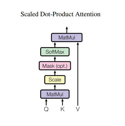
변환기가 사용하는 어텐션 기능은 Q(쿼리), K(키), V(값)의 세 가지 입력을 받습니다. 주의 가중치를 계산하는 데 사용되는 방정식은 다음과 같습니다.
\[\Large{Attention(Q, K, V) = softmax_k\left(\frac{QK^T}{\sqrt{d_k} }\right) V} \]
내적 주의는 깊이의 제곱근 계수로 조정됩니다. 이것은 깊이 값이 크면 내적(dot product)이 큰 크기로 커지기 때문에 softmax 함수를 밀어서 작은 그라디언트가 있는 곳에서 매우 단단한 softmax가 생성됩니다.
예를 들어, Q 와 K 의 평균이 0이고 분산이 1이라고 가정합니다. 행렬 곱셈의 평균은 0이고 분산은 dk 입니다. 따라서 dk 의 제곱근은 스케일링에 사용되므로 dk 값에 관계없이 일관된 분산을 얻습니다. 분산이 너무 낮으면 출력이 너무 평평하여 효과적으로 최적화할 수 없습니다. 분산이 너무 높으면 softmax가 초기화 시 포화되어 학습하기 어려울 수 있습니다.
마스크에 -1e9를 곱합니다(음의 무한대에 가까움). 이것은 마스크가 Q와 K의 스케일된 행렬 곱으로 합산되고 softmax 직전에 적용되기 때문에 수행됩니다. 목표는 이러한 셀을 0으로 만드는 것이며 softmax에 대한 큰 음수 입력은 출력에서 거의 0에 가깝습니다.
def scaled_dot_product_attention(q, k, v, mask):
  """Calculate the attention weights.
  q, k, v must have matching leading dimensions.
  k, v must have matching penultimate dimension, i.e.: seq_len_k = seq_len_v.
  The mask has different shapes depending on its type(padding or look ahead)
  but it must be broadcastable for addition.

  Args:
    q: query shape == (..., seq_len_q, depth)
    k: key shape == (..., seq_len_k, depth)
    v: value shape == (..., seq_len_v, depth_v)
    mask: Float tensor with shape broadcastable
          to (..., seq_len_q, seq_len_k). Defaults to None.

  Returns:
    output, attention_weights
  """

  matmul_qk = tf.matmul(q, k, transpose_b=True)  # (..., seq_len_q, seq_len_k)

  # scale matmul_qk
  dk = tf.cast(tf.shape(k)[-1], tf.float32)
  scaled_attention_logits = matmul_qk / tf.math.sqrt(dk)

  # add the mask to the scaled tensor.
  if mask is not None:
    scaled_attention_logits += (mask * -1e9)

  # softmax is normalized on the last axis (seq_len_k) so that the scores
  # add up to 1.
  attention_weights = tf.nn.softmax(scaled_attention_logits, axis=-1)  # (..., seq_len_q, seq_len_k)

  output = tf.matmul(attention_weights, v)  # (..., seq_len_q, depth_v)

  return output, attention_weights
softmax normalization이 K에 대해 수행되면 해당 값에 따라 Q에 부여되는 중요도가 결정됩니다.
출력은 주의 가중치와 V(값) 벡터의 곱을 나타냅니다. 이렇게 하면 집중하려는 토큰이 있는 그대로 유지되고 관련 없는 토큰이 플러시됩니다.
def print_out(q, k, v):
  temp_out, temp_attn = scaled_dot_product_attention(
      q, k, v, None)
  print('Attention weights are:')
  print(temp_attn)
  print('Output is:')
  print(temp_out)
np.set_printoptions(suppress=True)

temp_k = tf.constant([[10, 0, 0],
                      [0, 10, 0],
                      [0, 0, 10],
                      [0, 0, 10]], dtype=tf.float32)  # (4, 3)

temp_v = tf.constant([[1, 0],
                      [10, 0],
                      [100, 5],
                      [1000, 6]], dtype=tf.float32)  # (4, 2)

# This `query` aligns with the second `key`,
# so the second `value` is returned.
temp_q = tf.constant([[0, 10, 0]], dtype=tf.float32)  # (1, 3)
print_out(temp_q, temp_k, temp_v)
Attention weights are:
tf.Tensor([[0. 1. 0. 0.]], shape=(1, 4), dtype=float32)
Output is:
tf.Tensor([[10.  0.]], shape=(1, 2), dtype=float32)
# This query aligns with a repeated key (third and fourth),
# so all associated values get averaged.
temp_q = tf.constant([[0, 0, 10]], dtype=tf.float32)  # (1, 3)
print_out(temp_q, temp_k, temp_v)
Attention weights are:
tf.Tensor([[0.  0.  0.5 0.5]], shape=(1, 4), dtype=float32)
Output is:
tf.Tensor([[550.    5.5]], shape=(1, 2), dtype=float32)
# This query aligns equally with the first and second key,
# so their values get averaged.
temp_q = tf.constant([[10, 10, 0]], dtype=tf.float32)  # (1, 3)
print_out(temp_q, temp_k, temp_v)
Attention weights are:
tf.Tensor([[0.5 0.5 0.  0. ]], shape=(1, 4), dtype=float32)
Output is:
tf.Tensor([[5.5 0. ]], shape=(1, 2), dtype=float32)
모든 쿼리를 함께 전달합니다.
temp_q = tf.constant([[0, 0, 10],
                      [0, 10, 0],
                      [10, 10, 0]], dtype=tf.float32)  # (3, 3)
print_out(temp_q, temp_k, temp_v)
Attention weights are:
tf.Tensor(
[[0.  0.  0.5 0.5]
 [0.  1.  0.  0. ]
 [0.5 0.5 0.  0. ]], shape=(3, 4), dtype=float32)
Output is:
tf.Tensor(
[[550.    5.5]
 [ 10.    0. ]
 [  5.5   0. ]], shape=(3, 2), dtype=float32)
멀티 헤드 주의
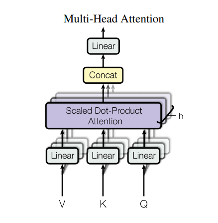
다중 머리 주의는 네 부분으로 구성됩니다.
- 선형 레이어.
- 확장된 내적 주의.
- 최종 선형 레이어.
각 다중 헤드 주의 블록은 3개의 입력을 받습니다. Q(쿼리), K(키), V(값). 이들은 다중 헤드 주의 기능 전에 선형(밀도) 레이어를 통해 배치됩니다.
위의 다이어그램에서 (K,Q,V) 는 각 주의 헤드에 대해 별도의 선형( Dense ) 레이어를 통과합니다. 단순성/효율성을 위해 아래 코드는 num_heads 배 더 많은 출력을 가진 단일 밀집 레이어를 사용하여 이것을 구현합니다. 어텐션 기능을 적용하기 전에 출력이 (batch, num_heads, ...) 모양으로 재배열됩니다.
위에서 정의한 scaled_dot_product_attention 함수는 효율성을 위해 브로드캐스트되는 단일 호출에 적용됩니다. 주의 단계에서는 적절한 마스크를 사용해야 합니다. 그런 다음 각 헤드에 대한 주의 출력이 연결되고( tf.transpose 및 tf.reshape 사용) 최종 Dense 레이어를 통과합니다.
하나의 주의 헤드 대신 Q, K 및 V가 여러 헤드로 분할됩니다. 모델이 서로 다른 위치에 있는 서로 다른 표현 부분 공간의 정보에 공동으로 주의를 기울일 수 있기 때문입니다. 분할 후 각 헤드는 감소된 차원을 가지므로 총 계산 비용은 전체 차원이 있는 단일 헤드 주의와 동일합니다.
class MultiHeadAttention(tf.keras.layers.Layer):
  def __init__(self, d_model, num_heads):
    super(MultiHeadAttention, self).__init__()
    self.num_heads = num_heads
    self.d_model = d_model

    assert d_model % self.num_heads == 0

    self.depth = d_model // self.num_heads

    self.wq = tf.keras.layers.Dense(d_model)
    self.wk = tf.keras.layers.Dense(d_model)
    self.wv = tf.keras.layers.Dense(d_model)

    self.dense = tf.keras.layers.Dense(d_model)

  def split_heads(self, x, batch_size):
    """Split the last dimension into (num_heads, depth).
    Transpose the result such that the shape is (batch_size, num_heads, seq_len, depth)
    """
    x = tf.reshape(x, (batch_size, -1, self.num_heads, self.depth))
    return tf.transpose(x, perm=[0, 2, 1, 3])

  def call(self, v, k, q, mask):
    batch_size = tf.shape(q)[0]

    q = self.wq(q)  # (batch_size, seq_len, d_model)
    k = self.wk(k)  # (batch_size, seq_len, d_model)
    v = self.wv(v)  # (batch_size, seq_len, d_model)

    q = self.split_heads(q, batch_size)  # (batch_size, num_heads, seq_len_q, depth)
    k = self.split_heads(k, batch_size)  # (batch_size, num_heads, seq_len_k, depth)
    v = self.split_heads(v, batch_size)  # (batch_size, num_heads, seq_len_v, depth)

    # scaled_attention.shape == (batch_size, num_heads, seq_len_q, depth)
    # attention_weights.shape == (batch_size, num_heads, seq_len_q, seq_len_k)
    scaled_attention, attention_weights = scaled_dot_product_attention(
        q, k, v, mask)

    scaled_attention = tf.transpose(scaled_attention, perm=[0, 2, 1, 3])  # (batch_size, seq_len_q, num_heads, depth)

    concat_attention = tf.reshape(scaled_attention,
                                  (batch_size, -1, self.d_model))  # (batch_size, seq_len_q, d_model)

    output = self.dense(concat_attention)  # (batch_size, seq_len_q, d_model)

    return output, attention_weights
시도할 MultiHeadAttention 레이어를 만듭니다. 시퀀스의 각 위치 y 에서 MultiHeadAttention 은 시퀀스의 다른 모든 위치에서 8개의 주의 헤드를 모두 실행하여 각 위치에서 동일한 길이의 새 벡터를 반환합니다.
temp_mha = MultiHeadAttention(d_model=512, num_heads=8)
y = tf.random.uniform((1, 60, 512))  # (batch_size, encoder_sequence, d_model)
out, attn = temp_mha(y, k=y, q=y, mask=None)
out.shape, attn.shape
(TensorShape([1, 60, 512]), TensorShape([1, 8, 60, 60]))
포인트 와이즈 피드포워드 네트워크
포인트 와이즈 피드 포워드 네트워크는 사이에 ReLU 활성화가 있는 두 개의 완전히 연결된 레이어로 구성됩니다.
def point_wise_feed_forward_network(d_model, dff):
  return tf.keras.Sequential([
      tf.keras.layers.Dense(dff, activation='relu'),  # (batch_size, seq_len, dff)
      tf.keras.layers.Dense(d_model)  # (batch_size, seq_len, d_model)
  ])
sample_ffn = point_wise_feed_forward_network(512, 2048)
sample_ffn(tf.random.uniform((64, 50, 512))).shape
TensorShape([64, 50, 512])
인코더 및 디코더
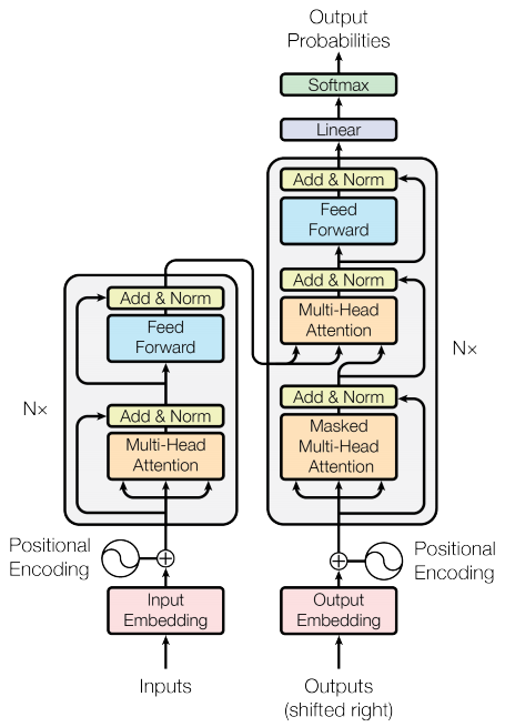
변환기 모델은 표준 시퀀스와 어텐션 모델 과 동일한 일반 패턴을 따릅니다.
- 입력 문장은 시퀀스의 각 토큰에 대한 출력을 생성하는
N인코더 계층을 통해 전달됩니다. - 디코더는 인코더의 출력과 자체 입력(자체 주의)에 주의하여 다음 단어를 예측합니다.
인코더 레이어
각 인코더 계층은 하위 계층으로 구성됩니다.
- 멀티 헤드 주의(패딩 마스크 포함)
- 포인트 와이즈 피드포워드 네트워크.
이러한 각 하위 계층에는 계층 정규화가 뒤따르는 잔여 연결이 있습니다. 잔차 연결은 심층 네트워크에서 사라지는 그래디언트 문제를 피하는 데 도움이 됩니다.
각 하위 계층의 출력은 LayerNorm(x + Sublayer(x)) 입니다. 정규화는 d_model (마지막) 축에서 수행됩니다. 변압기에는 N개의 인코더 레이어가 있습니다.
class EncoderLayer(tf.keras.layers.Layer):
  def __init__(self, d_model, num_heads, dff, rate=0.1):
    super(EncoderLayer, self).__init__()

    self.mha = MultiHeadAttention(d_model, num_heads)
    self.ffn = point_wise_feed_forward_network(d_model, dff)

    self.layernorm1 = tf.keras.layers.LayerNormalization(epsilon=1e-6)
    self.layernorm2 = tf.keras.layers.LayerNormalization(epsilon=1e-6)

    self.dropout1 = tf.keras.layers.Dropout(rate)
    self.dropout2 = tf.keras.layers.Dropout(rate)

  def call(self, x, training, mask):

    attn_output, _ = self.mha(x, x, x, mask)  # (batch_size, input_seq_len, d_model)
    attn_output = self.dropout1(attn_output, training=training)
    out1 = self.layernorm1(x + attn_output)  # (batch_size, input_seq_len, d_model)

    ffn_output = self.ffn(out1)  # (batch_size, input_seq_len, d_model)
    ffn_output = self.dropout2(ffn_output, training=training)
    out2 = self.layernorm2(out1 + ffn_output)  # (batch_size, input_seq_len, d_model)

    return out2
sample_encoder_layer = EncoderLayer(512, 8, 2048)

sample_encoder_layer_output = sample_encoder_layer(
    tf.random.uniform((64, 43, 512)), False, None)

sample_encoder_layer_output.shape  # (batch_size, input_seq_len, d_model)
TensorShape([64, 43, 512])
디코더 레이어
각 디코더 계층은 하위 계층으로 구성됩니다.
- 마스킹된 멀티 헤드 어텐션(미리보기 마스크 및 패딩 마스크 포함)
- 다중 헤드 주의(패딩 마스크 포함). V(값) 및 K(키)는 인코더 출력 을 입력으로 받습니다. Q(쿼리)는 마스크된 다중 헤드 주의 하위 계층에서 출력을 수신합니다.
- 포인트 와이즈 피드포워드 네트워크
이러한 각 하위 계층에는 계층 정규화가 뒤따르는 잔여 연결이 있습니다. 각 하위 계층의 출력은 LayerNorm(x + Sublayer(x)) 입니다. 정규화는 d_model (마지막) 축에서 수행됩니다.
변압기에는 N개의 디코더 레이어가 있습니다.
Q는 디코더의 첫 번째 주의 블록에서 출력을 수신하고 K는 인코더 출력을 수신하므로 주의 가중치는 인코더의 출력을 기반으로 디코더의 입력에 주어진 중요도를 나타냅니다. 즉, 디코더는 인코더 출력을 보고 자체 출력에 자가 참여하여 다음 토큰을 예측합니다. 위의 Scaled Dot Product Attention 섹션에서 데모를 참조하세요.
class DecoderLayer(tf.keras.layers.Layer):
  def __init__(self, d_model, num_heads, dff, rate=0.1):
    super(DecoderLayer, self).__init__()

    self.mha1 = MultiHeadAttention(d_model, num_heads)
    self.mha2 = MultiHeadAttention(d_model, num_heads)

    self.ffn = point_wise_feed_forward_network(d_model, dff)

    self.layernorm1 = tf.keras.layers.LayerNormalization(epsilon=1e-6)
    self.layernorm2 = tf.keras.layers.LayerNormalization(epsilon=1e-6)
    self.layernorm3 = tf.keras.layers.LayerNormalization(epsilon=1e-6)

    self.dropout1 = tf.keras.layers.Dropout(rate)
    self.dropout2 = tf.keras.layers.Dropout(rate)
    self.dropout3 = tf.keras.layers.Dropout(rate)

  def call(self, x, enc_output, training,
           look_ahead_mask, padding_mask):
    # enc_output.shape == (batch_size, input_seq_len, d_model)

    attn1, attn_weights_block1 = self.mha1(x, x, x, look_ahead_mask)  # (batch_size, target_seq_len, d_model)
    attn1 = self.dropout1(attn1, training=training)
    out1 = self.layernorm1(attn1 + x)

    attn2, attn_weights_block2 = self.mha2(
        enc_output, enc_output, out1, padding_mask)  # (batch_size, target_seq_len, d_model)
    attn2 = self.dropout2(attn2, training=training)
    out2 = self.layernorm2(attn2 + out1)  # (batch_size, target_seq_len, d_model)

    ffn_output = self.ffn(out2)  # (batch_size, target_seq_len, d_model)
    ffn_output = self.dropout3(ffn_output, training=training)
    out3 = self.layernorm3(ffn_output + out2)  # (batch_size, target_seq_len, d_model)

    return out3, attn_weights_block1, attn_weights_block2
sample_decoder_layer = DecoderLayer(512, 8, 2048)

sample_decoder_layer_output, _, _ = sample_decoder_layer(
    tf.random.uniform((64, 50, 512)), sample_encoder_layer_output,
    False, None, None)

sample_decoder_layer_output.shape  # (batch_size, target_seq_len, d_model)
TensorShape([64, 50, 512])
인코더
Encoder 는 다음으로 구성됩니다.
- 입력 임베딩
- 위치 인코딩
- N 인코더 레이어
위치 인코딩과 합산되는 임베딩을 통해 입력이 입력됩니다. 이 합산의 출력은 인코더 계층에 대한 입력입니다. 인코더의 출력은 디코더의 입력입니다.
class Encoder(tf.keras.layers.Layer):
  def __init__(self, num_layers, d_model, num_heads, dff, input_vocab_size,
               maximum_position_encoding, rate=0.1):
    super(Encoder, self).__init__()

    self.d_model = d_model
    self.num_layers = num_layers

    self.embedding = tf.keras.layers.Embedding(input_vocab_size, d_model)
    self.pos_encoding = positional_encoding(maximum_position_encoding,
                                            self.d_model)

    self.enc_layers = [EncoderLayer(d_model, num_heads, dff, rate)
                       for _ in range(num_layers)]

    self.dropout = tf.keras.layers.Dropout(rate)

  def call(self, x, training, mask):

    seq_len = tf.shape(x)[1]

    # adding embedding and position encoding.
    x = self.embedding(x)  # (batch_size, input_seq_len, d_model)
    x *= tf.math.sqrt(tf.cast(self.d_model, tf.float32))
    x += self.pos_encoding[:, :seq_len, :]

    x = self.dropout(x, training=training)

    for i in range(self.num_layers):
      x = self.enc_layers[i](x, training, mask)

    return x  # (batch_size, input_seq_len, d_model)
sample_encoder = Encoder(num_layers=2, d_model=512, num_heads=8,
                         dff=2048, input_vocab_size=8500,
                         maximum_position_encoding=10000)
temp_input = tf.random.uniform((64, 62), dtype=tf.int64, minval=0, maxval=200)

sample_encoder_output = sample_encoder(temp_input, training=False, mask=None)

print(sample_encoder_output.shape)  # (batch_size, input_seq_len, d_model)
(64, 62, 512)
디코더
Decoder 는 다음으로 구성됩니다.
- 출력 임베딩
- 위치 인코딩
- N 디코더 레이어
대상은 위치 인코딩과 합산되는 임베딩을 통해 배치됩니다. 이 합산의 출력은 디코더 계층에 대한 입력입니다. 디코더의 출력은 최종 선형 계층에 대한 입력입니다.
class Decoder(tf.keras.layers.Layer):
  def __init__(self, num_layers, d_model, num_heads, dff, target_vocab_size,
               maximum_position_encoding, rate=0.1):
    super(Decoder, self).__init__()

    self.d_model = d_model
    self.num_layers = num_layers

    self.embedding = tf.keras.layers.Embedding(target_vocab_size, d_model)
    self.pos_encoding = positional_encoding(maximum_position_encoding, d_model)

    self.dec_layers = [DecoderLayer(d_model, num_heads, dff, rate)
                       for _ in range(num_layers)]
    self.dropout = tf.keras.layers.Dropout(rate)

  def call(self, x, enc_output, training,
           look_ahead_mask, padding_mask):

    seq_len = tf.shape(x)[1]
    attention_weights = {}

    x = self.embedding(x)  # (batch_size, target_seq_len, d_model)
    x *= tf.math.sqrt(tf.cast(self.d_model, tf.float32))
    x += self.pos_encoding[:, :seq_len, :]

    x = self.dropout(x, training=training)

    for i in range(self.num_layers):
      x, block1, block2 = self.dec_layers[i](x, enc_output, training,
                                             look_ahead_mask, padding_mask)

      attention_weights[f'decoder_layer{i+1}_block1'] = block1
      attention_weights[f'decoder_layer{i+1}_block2'] = block2

    # x.shape == (batch_size, target_seq_len, d_model)
    return x, attention_weights
sample_decoder = Decoder(num_layers=2, d_model=512, num_heads=8,
                         dff=2048, target_vocab_size=8000,
                         maximum_position_encoding=5000)
temp_input = tf.random.uniform((64, 26), dtype=tf.int64, minval=0, maxval=200)

output, attn = sample_decoder(temp_input,
                              enc_output=sample_encoder_output,
                              training=False,
                              look_ahead_mask=None,
                              padding_mask=None)

output.shape, attn['decoder_layer2_block2'].shape
(TensorShape([64, 26, 512]), TensorShape([64, 8, 26, 62]))
변압기 만들기
Transformer는 인코더, 디코더 및 최종 선형 레이어로 구성됩니다. 디코더의 출력은 선형 레이어에 대한 입력이고 출력은 반환됩니다.
class Transformer(tf.keras.Model):
  def __init__(self, num_layers, d_model, num_heads, dff, input_vocab_size,
               target_vocab_size, pe_input, pe_target, rate=0.1):
    super().__init__()
    self.encoder = Encoder(num_layers, d_model, num_heads, dff,
                             input_vocab_size, pe_input, rate)

    self.decoder = Decoder(num_layers, d_model, num_heads, dff,
                           target_vocab_size, pe_target, rate)

    self.final_layer = tf.keras.layers.Dense(target_vocab_size)

  def call(self, inputs, training):
    # Keras models prefer if you pass all your inputs in the first argument
    inp, tar = inputs

    enc_padding_mask, look_ahead_mask, dec_padding_mask = self.create_masks(inp, tar)

    enc_output = self.encoder(inp, training, enc_padding_mask)  # (batch_size, inp_seq_len, d_model)

    # dec_output.shape == (batch_size, tar_seq_len, d_model)
    dec_output, attention_weights = self.decoder(
        tar, enc_output, training, look_ahead_mask, dec_padding_mask)

    final_output = self.final_layer(dec_output)  # (batch_size, tar_seq_len, target_vocab_size)

    return final_output, attention_weights

  def create_masks(self, inp, tar):
    # Encoder padding mask
    enc_padding_mask = create_padding_mask(inp)

    # Used in the 2nd attention block in the decoder.
    # This padding mask is used to mask the encoder outputs.
    dec_padding_mask = create_padding_mask(inp)

    # Used in the 1st attention block in the decoder.
    # It is used to pad and mask future tokens in the input received by
    # the decoder.
    look_ahead_mask = create_look_ahead_mask(tf.shape(tar)[1])
    dec_target_padding_mask = create_padding_mask(tar)
    look_ahead_mask = tf.maximum(dec_target_padding_mask, look_ahead_mask)

    return enc_padding_mask, look_ahead_mask, dec_padding_mask
sample_transformer = Transformer(
    num_layers=2, d_model=512, num_heads=8, dff=2048,
    input_vocab_size=8500, target_vocab_size=8000,
    pe_input=10000, pe_target=6000)

temp_input = tf.random.uniform((64, 38), dtype=tf.int64, minval=0, maxval=200)
temp_target = tf.random.uniform((64, 36), dtype=tf.int64, minval=0, maxval=200)

fn_out, _ = sample_transformer([temp_input, temp_target], training=False)

fn_out.shape  # (batch_size, tar_seq_len, target_vocab_size)
TensorShape([64, 36, 8000])
초매개변수 설정
이 예제를 작고 상대적으로 빠르게 유지하기 위해 num_layers, d_model, dff 의 값을 줄였습니다.
사용된 문서 에 설명된 기본 모델: num_layers=6, d_model=512, dff=2048 .
num_layers = 4
d_model = 128
dff = 512
num_heads = 8
dropout_rate = 0.1
옵티마이저
논문 의 공식에 따라 맞춤형 학습률 스케줄러와 함께 Adam 최적화 프로그램을 사용합니다.
\[\Large{lrate = d_{model}^{-0.5} * \min(step{\_}num^{-0.5}, step{\_}num \cdot warmup{\_}steps^{-1.5})}\]
class CustomSchedule(tf.keras.optimizers.schedules.LearningRateSchedule):
  def __init__(self, d_model, warmup_steps=4000):
    super(CustomSchedule, self).__init__()

    self.d_model = d_model
    self.d_model = tf.cast(self.d_model, tf.float32)

    self.warmup_steps = warmup_steps

  def __call__(self, step):
    arg1 = tf.math.rsqrt(step)
    arg2 = step * (self.warmup_steps ** -1.5)

    return tf.math.rsqrt(self.d_model) * tf.math.minimum(arg1, arg2)
learning_rate = CustomSchedule(d_model)

optimizer = tf.keras.optimizers.Adam(learning_rate, beta_1=0.9, beta_2=0.98,
                                     epsilon=1e-9)
temp_learning_rate_schedule = CustomSchedule(d_model)

plt.plot(temp_learning_rate_schedule(tf.range(40000, dtype=tf.float32)))
plt.ylabel("Learning Rate")
plt.xlabel("Train Step")
Text(0.5, 0, 'Train Step')

손실 및 측정항목
타겟 시퀀스가 패딩되기 때문에 손실을 계산할 때 패딩 마스크를 적용하는 것이 중요합니다.
loss_object = tf.keras.losses.SparseCategoricalCrossentropy(
    from_logits=True, reduction='none')
def loss_function(real, pred):
  mask = tf.math.logical_not(tf.math.equal(real, 0))
  loss_ = loss_object(real, pred)

  mask = tf.cast(mask, dtype=loss_.dtype)
  loss_ *= mask

  return tf.reduce_sum(loss_)/tf.reduce_sum(mask)


def accuracy_function(real, pred):
  accuracies = tf.equal(real, tf.argmax(pred, axis=2))

  mask = tf.math.logical_not(tf.math.equal(real, 0))
  accuracies = tf.math.logical_and(mask, accuracies)

  accuracies = tf.cast(accuracies, dtype=tf.float32)
  mask = tf.cast(mask, dtype=tf.float32)
  return tf.reduce_sum(accuracies)/tf.reduce_sum(mask)
train_loss = tf.keras.metrics.Mean(name='train_loss')
train_accuracy = tf.keras.metrics.Mean(name='train_accuracy')
훈련 및 체크포인트
transformer = Transformer(
    num_layers=num_layers,
    d_model=d_model,
    num_heads=num_heads,
    dff=dff,
    input_vocab_size=tokenizers.pt.get_vocab_size().numpy(),
    target_vocab_size=tokenizers.en.get_vocab_size().numpy(),
    pe_input=1000,
    pe_target=1000,
    rate=dropout_rate)
체크포인트 경로와 체크포인트 매니저를 생성합니다. 이것은 n epoch마다 체크포인트를 저장하는 데 사용됩니다.
checkpoint_path = "./checkpoints/train"

ckpt = tf.train.Checkpoint(transformer=transformer,
                           optimizer=optimizer)

ckpt_manager = tf.train.CheckpointManager(ckpt, checkpoint_path, max_to_keep=5)

# if a checkpoint exists, restore the latest checkpoint.
if ckpt_manager.latest_checkpoint:
  ckpt.restore(ckpt_manager.latest_checkpoint)
  print('Latest checkpoint restored!!')
타겟은 tar_inp와 tar_real로 나뉩니다. tar_inp는 디코더에 대한 입력으로 전달됩니다. tar_real 은 1만큼 이동한 동일한 입력입니다. tar_real 의 각 위치에서 tar_input 은 예측해야 하는 다음 토큰을 포함합니다.
예를 들어 sentence = "SOS 정글 속의 사자가 EOS를 자고 있다"
tar_inp = "SOS 정글에서 사자가 자고 있습니다"
tar_real = "정글의 사자가 잠든 EOS"
변환기는 자동 회귀 모델입니다. 변환기는 한 번에 한 부분씩 예측하고 지금까지의 출력을 사용하여 다음에 수행할 작업을 결정합니다.
훈련 중에 이 예제는 교사 강제를 사용합니다(예: 텍스트 생성 자습서 ). 교사 강제는 모델이 현재 시간 단계에서 예측하는 것과 상관없이 실제 출력을 다음 시간 단계로 전달합니다.
변환기가 각 토큰을 예측할 때 자체 주의 를 통해 입력 시퀀스의 이전 토큰을 보고 다음 토큰을 더 잘 예측할 수 있습니다.
모델이 예상 출력을 엿보는 것을 방지하기 위해 모델은 미리보기 마스크를 사용합니다.
EPOCHS = 20
# The @tf.function trace-compiles train_step into a TF graph for faster
# execution. The function specializes to the precise shape of the argument
# tensors. To avoid re-tracing due to the variable sequence lengths or variable
# batch sizes (the last batch is smaller), use input_signature to specify
# more generic shapes.

train_step_signature = [
    tf.TensorSpec(shape=(None, None), dtype=tf.int64),
    tf.TensorSpec(shape=(None, None), dtype=tf.int64),
]


@tf.function(input_signature=train_step_signature)
def train_step(inp, tar):
  tar_inp = tar[:, :-1]
  tar_real = tar[:, 1:]

  with tf.GradientTape() as tape:
    predictions, _ = transformer([inp, tar_inp],
                                 training = True)
    loss = loss_function(tar_real, predictions)

  gradients = tape.gradient(loss, transformer.trainable_variables)
  optimizer.apply_gradients(zip(gradients, transformer.trainable_variables))

  train_loss(loss)
  train_accuracy(accuracy_function(tar_real, predictions))
포르투갈어가 입력 언어로 사용되고 영어가 대상 언어입니다.
for epoch in range(EPOCHS):
  start = time.time()

  train_loss.reset_states()
  train_accuracy.reset_states()

  # inp -> portuguese, tar -> english
  for (batch, (inp, tar)) in enumerate(train_batches):
    train_step(inp, tar)

    if batch % 50 == 0:
      print(f'Epoch {epoch + 1} Batch {batch} Loss {train_loss.result():.4f} Accuracy {train_accuracy.result():.4f}')

  if (epoch + 1) % 5 == 0:
    ckpt_save_path = ckpt_manager.save()
    print(f'Saving checkpoint for epoch {epoch+1} at {ckpt_save_path}')

  print(f'Epoch {epoch + 1} Loss {train_loss.result():.4f} Accuracy {train_accuracy.result():.4f}')

  print(f'Time taken for 1 epoch: {time.time() - start:.2f} secs\n')
Epoch 1 Batch 0 Loss 8.8600 Accuracy 0.0000
Epoch 1 Batch 50 Loss 8.7935 Accuracy 0.0082
Epoch 1 Batch 100 Loss 8.6902 Accuracy 0.0273
Epoch 1 Batch 150 Loss 8.5769 Accuracy 0.0335
Epoch 1 Batch 200 Loss 8.4387 Accuracy 0.0365
Epoch 1 Batch 250 Loss 8.2718 Accuracy 0.0386
Epoch 1 Batch 300 Loss 8.0845 Accuracy 0.0412
Epoch 1 Batch 350 Loss 7.8877 Accuracy 0.0481
Epoch 1 Batch 400 Loss 7.7002 Accuracy 0.0552
Epoch 1 Batch 450 Loss 7.5304 Accuracy 0.0629
Epoch 1 Batch 500 Loss 7.3857 Accuracy 0.0702
Epoch 1 Batch 550 Loss 7.2542 Accuracy 0.0776
Epoch 1 Batch 600 Loss 7.1327 Accuracy 0.0851
Epoch 1 Batch 650 Loss 7.0164 Accuracy 0.0930
Epoch 1 Batch 700 Loss 6.9088 Accuracy 0.1003
Epoch 1 Batch 750 Loss 6.8080 Accuracy 0.1070
Epoch 1 Batch 800 Loss 6.7173 Accuracy 0.1129
Epoch 1 Loss 6.7021 Accuracy 0.1139
Time taken for 1 epoch: 58.85 secs

Epoch 2 Batch 0 Loss 5.2952 Accuracy 0.2221
Epoch 2 Batch 50 Loss 5.2513 Accuracy 0.2094
Epoch 2 Batch 100 Loss 5.2103 Accuracy 0.2140
Epoch 2 Batch 150 Loss 5.1780 Accuracy 0.2176
Epoch 2 Batch 200 Loss 5.1436 Accuracy 0.2218
Epoch 2 Batch 250 Loss 5.1173 Accuracy 0.2246
Epoch 2 Batch 300 Loss 5.0939 Accuracy 0.2269
Epoch 2 Batch 350 Loss 5.0719 Accuracy 0.2295
Epoch 2 Batch 400 Loss 5.0508 Accuracy 0.2318
Epoch 2 Batch 450 Loss 5.0308 Accuracy 0.2337
Epoch 2 Batch 500 Loss 5.0116 Accuracy 0.2353
Epoch 2 Batch 550 Loss 4.9897 Accuracy 0.2376
Epoch 2 Batch 600 Loss 4.9701 Accuracy 0.2394
Epoch 2 Batch 650 Loss 4.9543 Accuracy 0.2407
Epoch 2 Batch 700 Loss 4.9345 Accuracy 0.2425
Epoch 2 Batch 750 Loss 4.9169 Accuracy 0.2442
Epoch 2 Batch 800 Loss 4.9007 Accuracy 0.2455
Epoch 2 Loss 4.8988 Accuracy 0.2456
Time taken for 1 epoch: 45.69 secs

Epoch 3 Batch 0 Loss 4.7236 Accuracy 0.2578
Epoch 3 Batch 50 Loss 4.5860 Accuracy 0.2705
Epoch 3 Batch 100 Loss 4.5758 Accuracy 0.2723
Epoch 3 Batch 150 Loss 4.5789 Accuracy 0.2728
Epoch 3 Batch 200 Loss 4.5699 Accuracy 0.2737
Epoch 3 Batch 250 Loss 4.5529 Accuracy 0.2753
Epoch 3 Batch 300 Loss 4.5462 Accuracy 0.2753
Epoch 3 Batch 350 Loss 4.5377 Accuracy 0.2762
Epoch 3 Batch 400 Loss 4.5301 Accuracy 0.2764
Epoch 3 Batch 450 Loss 4.5155 Accuracy 0.2776
Epoch 3 Batch 500 Loss 4.5036 Accuracy 0.2787
Epoch 3 Batch 550 Loss 4.4950 Accuracy 0.2794
Epoch 3 Batch 600 Loss 4.4860 Accuracy 0.2804
Epoch 3 Batch 650 Loss 4.4753 Accuracy 0.2814
Epoch 3 Batch 700 Loss 4.4643 Accuracy 0.2823
Epoch 3 Batch 750 Loss 4.4530 Accuracy 0.2837
Epoch 3 Batch 800 Loss 4.4401 Accuracy 0.2852
Epoch 3 Loss 4.4375 Accuracy 0.2855
Time taken for 1 epoch: 45.96 secs

Epoch 4 Batch 0 Loss 3.9880 Accuracy 0.3285
Epoch 4 Batch 50 Loss 4.1496 Accuracy 0.3146
Epoch 4 Batch 100 Loss 4.1353 Accuracy 0.3146
Epoch 4 Batch 150 Loss 4.1263 Accuracy 0.3153
Epoch 4 Batch 200 Loss 4.1171 Accuracy 0.3165
Epoch 4 Batch 250 Loss 4.1144 Accuracy 0.3169
Epoch 4 Batch 300 Loss 4.0976 Accuracy 0.3190
Epoch 4 Batch 350 Loss 4.0848 Accuracy 0.3206
Epoch 4 Batch 400 Loss 4.0703 Accuracy 0.3228
Epoch 4 Batch 450 Loss 4.0569 Accuracy 0.3247
Epoch 4 Batch 500 Loss 4.0429 Accuracy 0.3265
Epoch 4 Batch 550 Loss 4.0231 Accuracy 0.3291
Epoch 4 Batch 600 Loss 4.0075 Accuracy 0.3311
Epoch 4 Batch 650 Loss 3.9933 Accuracy 0.3331
Epoch 4 Batch 700 Loss 3.9778 Accuracy 0.3353
Epoch 4 Batch 750 Loss 3.9625 Accuracy 0.3375
Epoch 4 Batch 800 Loss 3.9505 Accuracy 0.3393
Epoch 4 Loss 3.9483 Accuracy 0.3397
Time taken for 1 epoch: 45.59 secs

Epoch 5 Batch 0 Loss 3.7342 Accuracy 0.3712
Epoch 5 Batch 50 Loss 3.5723 Accuracy 0.3851
Epoch 5 Batch 100 Loss 3.5656 Accuracy 0.3861
Epoch 5 Batch 150 Loss 3.5706 Accuracy 0.3857
Epoch 5 Batch 200 Loss 3.5701 Accuracy 0.3863
Epoch 5 Batch 250 Loss 3.5621 Accuracy 0.3877
Epoch 5 Batch 300 Loss 3.5527 Accuracy 0.3887
Epoch 5 Batch 350 Loss 3.5429 Accuracy 0.3904
Epoch 5 Batch 400 Loss 3.5318 Accuracy 0.3923
Epoch 5 Batch 450 Loss 3.5238 Accuracy 0.3937
Epoch 5 Batch 500 Loss 3.5141 Accuracy 0.3949
Epoch 5 Batch 550 Loss 3.5066 Accuracy 0.3958
Epoch 5 Batch 600 Loss 3.4956 Accuracy 0.3974
Epoch 5 Batch 650 Loss 3.4876 Accuracy 0.3986
Epoch 5 Batch 700 Loss 3.4788 Accuracy 0.4000
Epoch 5 Batch 750 Loss 3.4676 Accuracy 0.4014
Epoch 5 Batch 800 Loss 3.4590 Accuracy 0.4027
Saving checkpoint for epoch 5 at ./checkpoints/train/ckpt-1
Epoch 5 Loss 3.4583 Accuracy 0.4029
Time taken for 1 epoch: 46.04 secs

Epoch 6 Batch 0 Loss 3.0131 Accuracy 0.4610
Epoch 6 Batch 50 Loss 3.1403 Accuracy 0.4404
Epoch 6 Batch 100 Loss 3.1320 Accuracy 0.4422
Epoch 6 Batch 150 Loss 3.1314 Accuracy 0.4425
Epoch 6 Batch 200 Loss 3.1450 Accuracy 0.4411
Epoch 6 Batch 250 Loss 3.1438 Accuracy 0.4405
Epoch 6 Batch 300 Loss 3.1306 Accuracy 0.4424
Epoch 6 Batch 350 Loss 3.1161 Accuracy 0.4445
Epoch 6 Batch 400 Loss 3.1097 Accuracy 0.4453
Epoch 6 Batch 450 Loss 3.0983 Accuracy 0.4469
Epoch 6 Batch 500 Loss 3.0900 Accuracy 0.4483
Epoch 6 Batch 550 Loss 3.0816 Accuracy 0.4496
Epoch 6 Batch 600 Loss 3.0740 Accuracy 0.4507
Epoch 6 Batch 650 Loss 3.0695 Accuracy 0.4514
Epoch 6 Batch 700 Loss 3.0602 Accuracy 0.4528
Epoch 6 Batch 750 Loss 3.0528 Accuracy 0.4539
Epoch 6 Batch 800 Loss 3.0436 Accuracy 0.4553
Epoch 6 Loss 3.0425 Accuracy 0.4554
Time taken for 1 epoch: 46.13 secs

Epoch 7 Batch 0 Loss 2.7147 Accuracy 0.4940
Epoch 7 Batch 50 Loss 2.7671 Accuracy 0.4863
Epoch 7 Batch 100 Loss 2.7369 Accuracy 0.4934
Epoch 7 Batch 150 Loss 2.7562 Accuracy 0.4909
Epoch 7 Batch 200 Loss 2.7441 Accuracy 0.4926
Epoch 7 Batch 250 Loss 2.7464 Accuracy 0.4929
Epoch 7 Batch 300 Loss 2.7430 Accuracy 0.4932
Epoch 7 Batch 350 Loss 2.7342 Accuracy 0.4944
Epoch 7 Batch 400 Loss 2.7271 Accuracy 0.4954
Epoch 7 Batch 450 Loss 2.7215 Accuracy 0.4963
Epoch 7 Batch 500 Loss 2.7157 Accuracy 0.4972
Epoch 7 Batch 550 Loss 2.7123 Accuracy 0.4978
Epoch 7 Batch 600 Loss 2.7071 Accuracy 0.4985
Epoch 7 Batch 650 Loss 2.7038 Accuracy 0.4990
Epoch 7 Batch 700 Loss 2.6979 Accuracy 0.5002
Epoch 7 Batch 750 Loss 2.6946 Accuracy 0.5007
Epoch 7 Batch 800 Loss 2.6923 Accuracy 0.5013
Epoch 7 Loss 2.6913 Accuracy 0.5015
Time taken for 1 epoch: 46.02 secs

Epoch 8 Batch 0 Loss 2.3681 Accuracy 0.5459
Epoch 8 Batch 50 Loss 2.4812 Accuracy 0.5260
Epoch 8 Batch 100 Loss 2.4682 Accuracy 0.5294
Epoch 8 Batch 150 Loss 2.4743 Accuracy 0.5287
Epoch 8 Batch 200 Loss 2.4625 Accuracy 0.5303
Epoch 8 Batch 250 Loss 2.4627 Accuracy 0.5303
Epoch 8 Batch 300 Loss 2.4624 Accuracy 0.5308
Epoch 8 Batch 350 Loss 2.4586 Accuracy 0.5314
Epoch 8 Batch 400 Loss 2.4532 Accuracy 0.5324
Epoch 8 Batch 450 Loss 2.4530 Accuracy 0.5326
Epoch 8 Batch 500 Loss 2.4508 Accuracy 0.5330
Epoch 8 Batch 550 Loss 2.4481 Accuracy 0.5338
Epoch 8 Batch 600 Loss 2.4455 Accuracy 0.5343
Epoch 8 Batch 650 Loss 2.4427 Accuracy 0.5348
Epoch 8 Batch 700 Loss 2.4399 Accuracy 0.5352
Epoch 8 Batch 750 Loss 2.4392 Accuracy 0.5353
Epoch 8 Batch 800 Loss 2.4367 Accuracy 0.5358
Epoch 8 Loss 2.4357 Accuracy 0.5360
Time taken for 1 epoch: 45.31 secs

Epoch 9 Batch 0 Loss 2.1790 Accuracy 0.5595
Epoch 9 Batch 50 Loss 2.2201 Accuracy 0.5676
Epoch 9 Batch 100 Loss 2.2420 Accuracy 0.5629
Epoch 9 Batch 150 Loss 2.2444 Accuracy 0.5623
Epoch 9 Batch 200 Loss 2.2535 Accuracy 0.5610
Epoch 9 Batch 250 Loss 2.2562 Accuracy 0.5603
Epoch 9 Batch 300 Loss 2.2572 Accuracy 0.5603
Epoch 9 Batch 350 Loss 2.2646 Accuracy 0.5592
Epoch 9 Batch 400 Loss 2.2624 Accuracy 0.5597
Epoch 9 Batch 450 Loss 2.2595 Accuracy 0.5601
Epoch 9 Batch 500 Loss 2.2598 Accuracy 0.5600
Epoch 9 Batch 550 Loss 2.2590 Accuracy 0.5602
Epoch 9 Batch 600 Loss 2.2563 Accuracy 0.5607
Epoch 9 Batch 650 Loss 2.2578 Accuracy 0.5606
Epoch 9 Batch 700 Loss 2.2550 Accuracy 0.5611
Epoch 9 Batch 750 Loss 2.2536 Accuracy 0.5614
Epoch 9 Batch 800 Loss 2.2511 Accuracy 0.5618
Epoch 9 Loss 2.2503 Accuracy 0.5620
Time taken for 1 epoch: 44.87 secs

Epoch 10 Batch 0 Loss 2.0921 Accuracy 0.5928
Epoch 10 Batch 50 Loss 2.1196 Accuracy 0.5788
Epoch 10 Batch 100 Loss 2.0969 Accuracy 0.5828
Epoch 10 Batch 150 Loss 2.0954 Accuracy 0.5834
Epoch 10 Batch 200 Loss 2.0965 Accuracy 0.5827
Epoch 10 Batch 250 Loss 2.1029 Accuracy 0.5822
Epoch 10 Batch 300 Loss 2.0999 Accuracy 0.5827
Epoch 10 Batch 350 Loss 2.1007 Accuracy 0.5825
Epoch 10 Batch 400 Loss 2.1011 Accuracy 0.5825
Epoch 10 Batch 450 Loss 2.1020 Accuracy 0.5826
Epoch 10 Batch 500 Loss 2.0977 Accuracy 0.5831
Epoch 10 Batch 550 Loss 2.0984 Accuracy 0.5831
Epoch 10 Batch 600 Loss 2.0985 Accuracy 0.5832
Epoch 10 Batch 650 Loss 2.1006 Accuracy 0.5830
Epoch 10 Batch 700 Loss 2.1017 Accuracy 0.5829
Epoch 10 Batch 750 Loss 2.1058 Accuracy 0.5825
Epoch 10 Batch 800 Loss 2.1059 Accuracy 0.5825
Saving checkpoint for epoch 10 at ./checkpoints/train/ckpt-2
Epoch 10 Loss 2.1060 Accuracy 0.5825
Time taken for 1 epoch: 45.06 secs

Epoch 11 Batch 0 Loss 2.1150 Accuracy 0.5829
Epoch 11 Batch 50 Loss 1.9694 Accuracy 0.6017
Epoch 11 Batch 100 Loss 1.9746 Accuracy 0.6007
Epoch 11 Batch 150 Loss 1.9787 Accuracy 0.5996
Epoch 11 Batch 200 Loss 1.9798 Accuracy 0.5992
Epoch 11 Batch 250 Loss 1.9781 Accuracy 0.5998
Epoch 11 Batch 300 Loss 1.9772 Accuracy 0.5999
Epoch 11 Batch 350 Loss 1.9807 Accuracy 0.5995
Epoch 11 Batch 400 Loss 1.9836 Accuracy 0.5990
Epoch 11 Batch 450 Loss 1.9854 Accuracy 0.5986
Epoch 11 Batch 500 Loss 1.9832 Accuracy 0.5993
Epoch 11 Batch 550 Loss 1.9828 Accuracy 0.5993
Epoch 11 Batch 600 Loss 1.9812 Accuracy 0.5996
Epoch 11 Batch 650 Loss 1.9822 Accuracy 0.5996
Epoch 11 Batch 700 Loss 1.9825 Accuracy 0.5997
Epoch 11 Batch 750 Loss 1.9848 Accuracy 0.5994
Epoch 11 Batch 800 Loss 1.9883 Accuracy 0.5990
Epoch 11 Loss 1.9891 Accuracy 0.5989
Time taken for 1 epoch: 44.58 secs

Epoch 12 Batch 0 Loss 1.8522 Accuracy 0.6168
Epoch 12 Batch 50 Loss 1.8462 Accuracy 0.6167
Epoch 12 Batch 100 Loss 1.8434 Accuracy 0.6191
Epoch 12 Batch 150 Loss 1.8506 Accuracy 0.6189
Epoch 12 Batch 200 Loss 1.8582 Accuracy 0.6178
Epoch 12 Batch 250 Loss 1.8732 Accuracy 0.6155
Epoch 12 Batch 300 Loss 1.8725 Accuracy 0.6159
Epoch 12 Batch 350 Loss 1.8708 Accuracy 0.6163
Epoch 12 Batch 400 Loss 1.8696 Accuracy 0.6164
Epoch 12 Batch 450 Loss 1.8696 Accuracy 0.6168
Epoch 12 Batch 500 Loss 1.8748 Accuracy 0.6160
Epoch 12 Batch 550 Loss 1.8793 Accuracy 0.6153
Epoch 12 Batch 600 Loss 1.8826 Accuracy 0.6149
Epoch 12 Batch 650 Loss 1.8851 Accuracy 0.6145
Epoch 12 Batch 700 Loss 1.8878 Accuracy 0.6143
Epoch 12 Batch 750 Loss 1.8881 Accuracy 0.6142
Epoch 12 Batch 800 Loss 1.8906 Accuracy 0.6139
Epoch 12 Loss 1.8919 Accuracy 0.6137
Time taken for 1 epoch: 44.87 secs

Epoch 13 Batch 0 Loss 1.7038 Accuracy 0.6438
Epoch 13 Batch 50 Loss 1.7587 Accuracy 0.6309
Epoch 13 Batch 100 Loss 1.7641 Accuracy 0.6313
Epoch 13 Batch 150 Loss 1.7736 Accuracy 0.6299
Epoch 13 Batch 200 Loss 1.7743 Accuracy 0.6299
Epoch 13 Batch 250 Loss 1.7787 Accuracy 0.6293
Epoch 13 Batch 300 Loss 1.7820 Accuracy 0.6286
Epoch 13 Batch 350 Loss 1.7890 Accuracy 0.6276
Epoch 13 Batch 400 Loss 1.7963 Accuracy 0.6264
Epoch 13 Batch 450 Loss 1.7984 Accuracy 0.6261
Epoch 13 Batch 500 Loss 1.8014 Accuracy 0.6256
Epoch 13 Batch 550 Loss 1.8018 Accuracy 0.6255
Epoch 13 Batch 600 Loss 1.8033 Accuracy 0.6253
Epoch 13 Batch 650 Loss 1.8057 Accuracy 0.6250
Epoch 13 Batch 700 Loss 1.8100 Accuracy 0.6246
Epoch 13 Batch 750 Loss 1.8123 Accuracy 0.6244
Epoch 13 Batch 800 Loss 1.8123 Accuracy 0.6246
Epoch 13 Loss 1.8123 Accuracy 0.6246
Time taken for 1 epoch: 45.34 secs

Epoch 14 Batch 0 Loss 2.0031 Accuracy 0.5889
Epoch 14 Batch 50 Loss 1.6906 Accuracy 0.6432
Epoch 14 Batch 100 Loss 1.7077 Accuracy 0.6407
Epoch 14 Batch 150 Loss 1.7113 Accuracy 0.6401
Epoch 14 Batch 200 Loss 1.7192 Accuracy 0.6382
Epoch 14 Batch 250 Loss 1.7220 Accuracy 0.6377
Epoch 14 Batch 300 Loss 1.7222 Accuracy 0.6376
Epoch 14 Batch 350 Loss 1.7250 Accuracy 0.6372
Epoch 14 Batch 400 Loss 1.7220 Accuracy 0.6377
Epoch 14 Batch 450 Loss 1.7209 Accuracy 0.6380
Epoch 14 Batch 500 Loss 1.7248 Accuracy 0.6377
Epoch 14 Batch 550 Loss 1.7264 Accuracy 0.6374
Epoch 14 Batch 600 Loss 1.7283 Accuracy 0.6373
Epoch 14 Batch 650 Loss 1.7307 Accuracy 0.6372
Epoch 14 Batch 700 Loss 1.7334 Accuracy 0.6367
Epoch 14 Batch 750 Loss 1.7372 Accuracy 0.6362
Epoch 14 Batch 800 Loss 1.7398 Accuracy 0.6358
Epoch 14 Loss 1.7396 Accuracy 0.6358
Time taken for 1 epoch: 46.00 secs

Epoch 15 Batch 0 Loss 1.6520 Accuracy 0.6395
Epoch 15 Batch 50 Loss 1.6565 Accuracy 0.6480
Epoch 15 Batch 100 Loss 1.6396 Accuracy 0.6495
Epoch 15 Batch 150 Loss 1.6473 Accuracy 0.6488
Epoch 15 Batch 200 Loss 1.6486 Accuracy 0.6488
Epoch 15 Batch 250 Loss 1.6539 Accuracy 0.6483
Epoch 15 Batch 300 Loss 1.6595 Accuracy 0.6473
Epoch 15 Batch 350 Loss 1.6591 Accuracy 0.6472
Epoch 15 Batch 400 Loss 1.6584 Accuracy 0.6470
Epoch 15 Batch 450 Loss 1.6614 Accuracy 0.6467
Epoch 15 Batch 500 Loss 1.6617 Accuracy 0.6468
Epoch 15 Batch 550 Loss 1.6648 Accuracy 0.6464
Epoch 15 Batch 600 Loss 1.6680 Accuracy 0.6459
Epoch 15 Batch 650 Loss 1.6688 Accuracy 0.6459
Epoch 15 Batch 700 Loss 1.6714 Accuracy 0.6456
Epoch 15 Batch 750 Loss 1.6756 Accuracy 0.6450
Epoch 15 Batch 800 Loss 1.6790 Accuracy 0.6445
Saving checkpoint for epoch 15 at ./checkpoints/train/ckpt-3
Epoch 15 Loss 1.6786 Accuracy 0.6446
Time taken for 1 epoch: 46.56 secs

Epoch 16 Batch 0 Loss 1.5922 Accuracy 0.6547
Epoch 16 Batch 50 Loss 1.5757 Accuracy 0.6599
Epoch 16 Batch 100 Loss 1.5844 Accuracy 0.6591
Epoch 16 Batch 150 Loss 1.5927 Accuracy 0.6579
Epoch 16 Batch 200 Loss 1.5944 Accuracy 0.6575
Epoch 16 Batch 250 Loss 1.5972 Accuracy 0.6571
Epoch 16 Batch 300 Loss 1.5999 Accuracy 0.6568
Epoch 16 Batch 350 Loss 1.6029 Accuracy 0.6561
Epoch 16 Batch 400 Loss 1.6053 Accuracy 0.6558
Epoch 16 Batch 450 Loss 1.6056 Accuracy 0.6557
Epoch 16 Batch 500 Loss 1.6094 Accuracy 0.6553
Epoch 16 Batch 550 Loss 1.6125 Accuracy 0.6548
Epoch 16 Batch 600 Loss 1.6149 Accuracy 0.6543
Epoch 16 Batch 650 Loss 1.6171 Accuracy 0.6541
Epoch 16 Batch 700 Loss 1.6201 Accuracy 0.6537
Epoch 16 Batch 750 Loss 1.6229 Accuracy 0.6533
Epoch 16 Batch 800 Loss 1.6252 Accuracy 0.6531
Epoch 16 Loss 1.6253 Accuracy 0.6531
Time taken for 1 epoch: 45.84 secs

Epoch 17 Batch 0 Loss 1.6605 Accuracy 0.6482
Epoch 17 Batch 50 Loss 1.5219 Accuracy 0.6692
Epoch 17 Batch 100 Loss 1.5292 Accuracy 0.6681
Epoch 17 Batch 150 Loss 1.5324 Accuracy 0.6674
Epoch 17 Batch 200 Loss 1.5379 Accuracy 0.6666
Epoch 17 Batch 250 Loss 1.5416 Accuracy 0.6656
Epoch 17 Batch 300 Loss 1.5480 Accuracy 0.6646
Epoch 17 Batch 350 Loss 1.5522 Accuracy 0.6639
Epoch 17 Batch 400 Loss 1.5556 Accuracy 0.6634
Epoch 17 Batch 450 Loss 1.5567 Accuracy 0.6634
Epoch 17 Batch 500 Loss 1.5606 Accuracy 0.6629
Epoch 17 Batch 550 Loss 1.5641 Accuracy 0.6624
Epoch 17 Batch 600 Loss 1.5659 Accuracy 0.6621
Epoch 17 Batch 650 Loss 1.5685 Accuracy 0.6618
Epoch 17 Batch 700 Loss 1.5716 Accuracy 0.6614
Epoch 17 Batch 750 Loss 1.5748 Accuracy 0.6610
Epoch 17 Batch 800 Loss 1.5764 Accuracy 0.6609
Epoch 17 Loss 1.5773 Accuracy 0.6607
Time taken for 1 epoch: 45.01 secs

Epoch 18 Batch 0 Loss 1.5065 Accuracy 0.6638
Epoch 18 Batch 50 Loss 1.4985 Accuracy 0.6713
Epoch 18 Batch 100 Loss 1.4979 Accuracy 0.6721
Epoch 18 Batch 150 Loss 1.5022 Accuracy 0.6712
Epoch 18 Batch 200 Loss 1.5012 Accuracy 0.6714
Epoch 18 Batch 250 Loss 1.5000 Accuracy 0.6716
Epoch 18 Batch 300 Loss 1.5044 Accuracy 0.6710
Epoch 18 Batch 350 Loss 1.5019 Accuracy 0.6719
Epoch 18 Batch 400 Loss 1.5053 Accuracy 0.6713
Epoch 18 Batch 450 Loss 1.5091 Accuracy 0.6707
Epoch 18 Batch 500 Loss 1.5131 Accuracy 0.6701
Epoch 18 Batch 550 Loss 1.5152 Accuracy 0.6698
Epoch 18 Batch 600 Loss 1.5177 Accuracy 0.6694
Epoch 18 Batch 650 Loss 1.5211 Accuracy 0.6689
Epoch 18 Batch 700 Loss 1.5246 Accuracy 0.6684
Epoch 18 Batch 750 Loss 1.5251 Accuracy 0.6685
Epoch 18 Batch 800 Loss 1.5302 Accuracy 0.6678
Epoch 18 Loss 1.5314 Accuracy 0.6675
Time taken for 1 epoch: 44.91 secs

Epoch 19 Batch 0 Loss 1.2939 Accuracy 0.7080
Epoch 19 Batch 50 Loss 1.4311 Accuracy 0.6839
Epoch 19 Batch 100 Loss 1.4424 Accuracy 0.6812
Epoch 19 Batch 150 Loss 1.4520 Accuracy 0.6799
Epoch 19 Batch 200 Loss 1.4604 Accuracy 0.6782
Epoch 19 Batch 250 Loss 1.4606 Accuracy 0.6783
Epoch 19 Batch 300 Loss 1.4627 Accuracy 0.6783
Epoch 19 Batch 350 Loss 1.4664 Accuracy 0.6777
Epoch 19 Batch 400 Loss 1.4720 Accuracy 0.6769
Epoch 19 Batch 450 Loss 1.4742 Accuracy 0.6764
Epoch 19 Batch 500 Loss 1.4772 Accuracy 0.6760
Epoch 19 Batch 550 Loss 1.4784 Accuracy 0.6759
Epoch 19 Batch 600 Loss 1.4807 Accuracy 0.6756
Epoch 19 Batch 650 Loss 1.4846 Accuracy 0.6750
Epoch 19 Batch 700 Loss 1.4877 Accuracy 0.6747
Epoch 19 Batch 750 Loss 1.4890 Accuracy 0.6745
Epoch 19 Batch 800 Loss 1.4918 Accuracy 0.6741
Epoch 19 Loss 1.4924 Accuracy 0.6740
Time taken for 1 epoch: 45.24 secs

Epoch 20 Batch 0 Loss 1.3994 Accuracy 0.6883
Epoch 20 Batch 50 Loss 1.3894 Accuracy 0.6911
Epoch 20 Batch 100 Loss 1.4050 Accuracy 0.6889
Epoch 20 Batch 150 Loss 1.4108 Accuracy 0.6883
Epoch 20 Batch 200 Loss 1.4111 Accuracy 0.6876
Epoch 20 Batch 250 Loss 1.4121 Accuracy 0.6871
Epoch 20 Batch 300 Loss 1.4179 Accuracy 0.6859
Epoch 20 Batch 350 Loss 1.4182 Accuracy 0.6857
Epoch 20 Batch 400 Loss 1.4212 Accuracy 0.6851
Epoch 20 Batch 450 Loss 1.4282 Accuracy 0.6837
Epoch 20 Batch 500 Loss 1.4296 Accuracy 0.6833
Epoch 20 Batch 550 Loss 1.4343 Accuracy 0.6826
Epoch 20 Batch 600 Loss 1.4375 Accuracy 0.6822
Epoch 20 Batch 650 Loss 1.4413 Accuracy 0.6817
Epoch 20 Batch 700 Loss 1.4464 Accuracy 0.6809
Epoch 20 Batch 750 Loss 1.4491 Accuracy 0.6805
Epoch 20 Batch 800 Loss 1.4530 Accuracy 0.6799
Saving checkpoint for epoch 20 at ./checkpoints/train/ckpt-4
Epoch 20 Loss 1.4533 Accuracy 0.6799
Time taken for 1 epoch: 45.84 secs
추론 실행
추론에는 다음 단계가 사용됩니다.
- 포르투갈어 토크나이저(
tokenizers.pt)를 사용하여 입력 문장을 인코딩합니다. 인코더 입력입니다. - 디코더 입력은
[START]토큰으로 초기화됩니다. - 패딩 마스크와 미리보기 마스크를 계산합니다.
- 그런 다음
decoder는encoder output과 자체 출력(셀프 어텐션)을 확인하여 예측을 출력합니다. - 예측된 토큰을 디코더 입력에 연결하고 디코더에 전달합니다.
- 이 접근 방식에서 디코더는 예측한 이전 토큰을 기반으로 다음 토큰을 예측합니다.
class Translator(tf.Module):
  def __init__(self, tokenizers, transformer):
    self.tokenizers = tokenizers
    self.transformer = transformer

  def __call__(self, sentence, max_length=20):
    # input sentence is portuguese, hence adding the start and end token
    assert isinstance(sentence, tf.Tensor)
    if len(sentence.shape) == 0:
      sentence = sentence[tf.newaxis]

    sentence = self.tokenizers.pt.tokenize(sentence).to_tensor()

    encoder_input = sentence

    # as the target is english, the first token to the transformer should be the
    # english start token.
    start_end = self.tokenizers.en.tokenize([''])[0]
    start = start_end[0][tf.newaxis]
    end = start_end[1][tf.newaxis]

    # `tf.TensorArray` is required here (instead of a python list) so that the
    # dynamic-loop can be traced by `tf.function`.
    output_array = tf.TensorArray(dtype=tf.int64, size=0, dynamic_size=True)
    output_array = output_array.write(0, start)

    for i in tf.range(max_length):
      output = tf.transpose(output_array.stack())
      predictions, _ = self.transformer([encoder_input, output], training=False)

      # select the last token from the seq_len dimension
      predictions = predictions[:, -1:, :]  # (batch_size, 1, vocab_size)

      predicted_id = tf.argmax(predictions, axis=-1)

      # concatentate the predicted_id to the output which is given to the decoder
      # as its input.
      output_array = output_array.write(i+1, predicted_id[0])

      if predicted_id == end:
        break

    output = tf.transpose(output_array.stack())
    # output.shape (1, tokens)
    text = tokenizers.en.detokenize(output)[0]  # shape: ()

    tokens = tokenizers.en.lookup(output)[0]

    # `tf.function` prevents us from using the attention_weights that were
    # calculated on the last iteration of the loop. So recalculate them outside
    # the loop.
    _, attention_weights = self.transformer([encoder_input, output[:,:-1]], training=False)

    return text, tokens, attention_weights
이 Translator 클래스의 인스턴스를 만들고 몇 번 시도해 보십시오.
translator = Translator(tokenizers, transformer)
def print_translation(sentence, tokens, ground_truth):
  print(f'{"Input:":15s}: {sentence}')
  print(f'{"Prediction":15s}: {tokens.numpy().decode("utf-8")}')
  print(f'{"Ground truth":15s}: {ground_truth}')
sentence = "este é um problema que temos que resolver."
ground_truth = "this is a problem we have to solve ."

translated_text, translated_tokens, attention_weights = translator(
    tf.constant(sentence))
print_translation(sentence, translated_text, ground_truth)
Input:         : este é um problema que temos que resolver.
Prediction     : this is a problem that we have to solve .
Ground truth   : this is a problem we have to solve .
sentence = "os meus vizinhos ouviram sobre esta ideia."
ground_truth = "and my neighboring homes heard about this idea ."

translated_text, translated_tokens, attention_weights = translator(
    tf.constant(sentence))
print_translation(sentence, translated_text, ground_truth)
Input:         : os meus vizinhos ouviram sobre esta ideia.
Prediction     : my neighbors heard about this idea .
Ground truth   : and my neighboring homes heard about this idea .
sentence = "vou então muito rapidamente partilhar convosco algumas histórias de algumas coisas mágicas que aconteceram."
ground_truth = "so i \'ll just share with you some stories very quickly of some magical things that have happened ."

translated_text, translated_tokens, attention_weights = translator(
    tf.constant(sentence))
print_translation(sentence, translated_text, ground_truth)
Input:         : vou então muito rapidamente partilhar convosco algumas histórias de algumas coisas mágicas que aconteceram.
Prediction     : so i ' m going to share with you a few stories of some magic things that have happened .
Ground truth   : so i 'll just share with you some stories very quickly of some magical things that have happened .
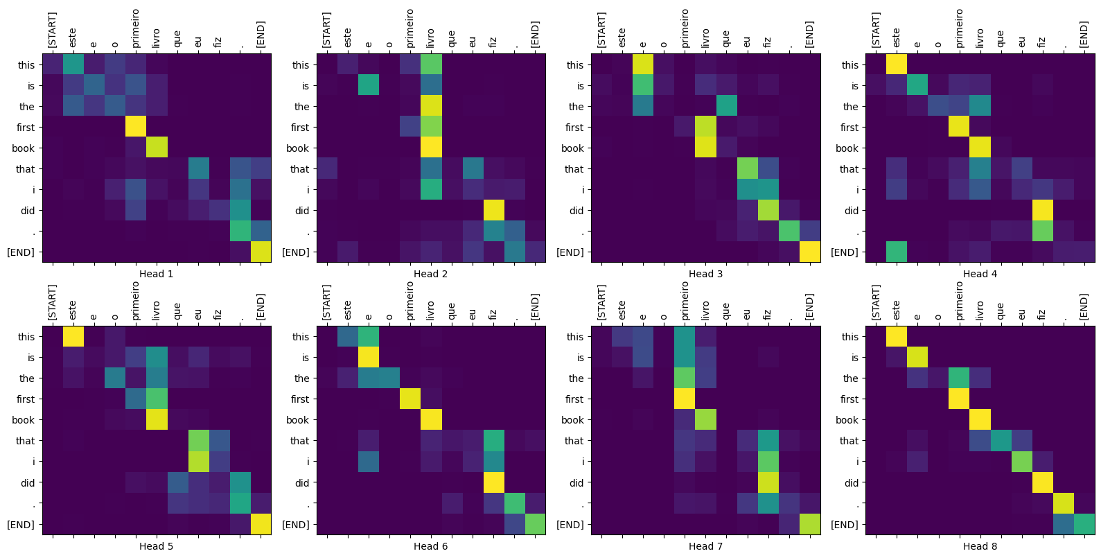
주의 플롯
Translator 클래스는 모델의 내부 작업을 시각화하는 데 사용할 수 있는 어텐션 맵의 사전을 반환합니다.
sentence = "este é o primeiro livro que eu fiz."
ground_truth = "this is the first book i've ever done."

translated_text, translated_tokens, attention_weights = translator(
    tf.constant(sentence))
print_translation(sentence, translated_text, ground_truth)
Input:         : este é o primeiro livro que eu fiz.
Prediction     : this is the first book that i did .
Ground truth   : this is the first book i've ever done.
def plot_attention_head(in_tokens, translated_tokens, attention):
  # The plot is of the attention when a token was generated.
  # The model didn't generate `<START>` in the output. Skip it.
  translated_tokens = translated_tokens[1:]

  ax = plt.gca()
  ax.matshow(attention)
  ax.set_xticks(range(len(in_tokens)))
  ax.set_yticks(range(len(translated_tokens)))

  labels = [label.decode('utf-8') for label in in_tokens.numpy()]
  ax.set_xticklabels(
      labels, rotation=90)

  labels = [label.decode('utf-8') for label in translated_tokens.numpy()]
  ax.set_yticklabels(labels)
head = 0
# shape: (batch=1, num_heads, seq_len_q, seq_len_k)
attention_heads = tf.squeeze(
  attention_weights['decoder_layer4_block2'], 0)
attention = attention_heads[head]
attention.shape
TensorShape([10, 11])
in_tokens = tf.convert_to_tensor([sentence])
in_tokens = tokenizers.pt.tokenize(in_tokens).to_tensor()
in_tokens = tokenizers.pt.lookup(in_tokens)[0]
in_tokens
<tf.Tensor: shape=(11,), dtype=string, numpy=
array([b'[START]', b'este', b'e', b'o', b'primeiro', b'livro', b'que',
       b'eu', b'fiz', b'.', b'[END]'], dtype=object)>
translated_tokens
<tf.Tensor: shape=(11,), dtype=string, numpy=
array([b'[START]', b'this', b'is', b'the', b'first', b'book', b'that',
       b'i', b'did', b'.', b'[END]'], dtype=object)>
plot_attention_head(in_tokens, translated_tokens, attention)

def plot_attention_weights(sentence, translated_tokens, attention_heads):
  in_tokens = tf.convert_to_tensor([sentence])
  in_tokens = tokenizers.pt.tokenize(in_tokens).to_tensor()
  in_tokens = tokenizers.pt.lookup(in_tokens)[0]
  in_tokens

  fig = plt.figure(figsize=(16, 8))

  for h, head in enumerate(attention_heads):
    ax = fig.add_subplot(2, 4, h+1)

    plot_attention_head(in_tokens, translated_tokens, head)

    ax.set_xlabel(f'Head {h+1}')

  plt.tight_layout()
  plt.show()
plot_attention_weights(sentence, translated_tokens,
                       attention_weights['decoder_layer4_block2'][0])

모델은 익숙하지 않은 단어를 잘합니다. "트리케라톱스" 또는 "백과사전"은 입력 데이터 세트에 없으며 모델은 공유 어휘 없이도 거의 음역하는 방법을 학습합니다.
sentence = "Eu li sobre triceratops na enciclopédia."
ground_truth = "I read about triceratops in the encyclopedia."

translated_text, translated_tokens, attention_weights = translator(
    tf.constant(sentence))
print_translation(sentence, translated_text, ground_truth)

plot_attention_weights(sentence, translated_tokens,
                       attention_weights['decoder_layer4_block2'][0])
Input:         : Eu li sobre triceratops na enciclopédia.
Prediction     : i read about trigatotys in the encyclopedia .
Ground truth   : I read about triceratops in the encyclopedia.

내 보내다
해당 추론 모델이 작동 중이므로 다음에는 이를 tf.saved_model 로 내보냅니다.
그렇게 하려면 이번에는 __call__ 메서드에 tf.function 을 사용하여 또 다른 tf.Module 하위 클래스로 래핑합니다.
class ExportTranslator(tf.Module):
  def __init__(self, translator):
    self.translator = translator

  @tf.function(input_signature=[tf.TensorSpec(shape=[], dtype=tf.string)])
  def __call__(self, sentence):
    (result,
     tokens,
     attention_weights) = self.translator(sentence, max_length=100)

    return result
위의 tf.function 에서는 출력 문장만 반환됩니다. tf.function 의 엄격하지 않은 실행 덕분에 불필요한 값은 절대 계산되지 않습니다.
translator = ExportTranslator(translator)
모델이 tf.argmax 를 사용하여 예측을 디코딩하기 때문에 예측은 결정적입니다. 원래 모델과 SavedModel 모델에서 다시 로드된 모델은 동일한 예측을 제공해야 합니다.
translator("este é o primeiro livro que eu fiz.").numpy()
b'this is the first book that i did .'
tf.saved_model.save(translator, export_dir='translator')
2022-02-04 13:19:17.308292: W tensorflow/python/util/util.cc:368] Sets are not currently considered sequences, but this may change in the future, so consider avoiding using them.
WARNING:absl:Found untraced functions such as embedding_4_layer_call_fn, embedding_4_layer_call_and_return_conditional_losses, dropout_37_layer_call_fn, dropout_37_layer_call_and_return_conditional_losses, embedding_5_layer_call_fn while saving (showing 5 of 224). These functions will not be directly callable after loading.
reloaded = tf.saved_model.load('translator')
reloaded("este é o primeiro livro que eu fiz.").numpy()
b'this is the first book that i did .'
요약
이 자습서에서는 위치 인코딩, 다중 헤드 주의, 마스킹의 중요성 및 변환기를 만드는 방법에 대해 배웠습니다.
다른 데이터 세트를 사용하여 변환기를 훈련시키십시오. 위의 하이퍼파라미터를 변경하여 기본 변환기 또는 변환기 XL을 생성할 수도 있습니다. 여기에 정의된 레이어를 사용하여 BERT 를 생성하고 최첨단 모델을 훈련할 수도 있습니다. 또한 더 나은 예측을 위해 빔 검색을 구현할 수 있습니다.