
| | |  GitHub पर स्रोत देखें GitHub पर स्रोत देखें | |
अवलोकन
डिब्बाबंद अनुमानक विशिष्ट उपयोग के मामलों के लिए टीएफएल मॉडल को प्रशिक्षित करने के त्वरित और आसान तरीके हैं। यह मार्गदर्शिका TFL डिब्बाबंद अनुमानक बनाने के लिए आवश्यक चरणों की रूपरेखा तैयार करती है।
सेट अप
TF जाली पैकेज स्थापित करना:
pip install tensorflow-lattice
आवश्यक पैकेज आयात करना:
import tensorflow as tf

import copy
import logging
import numpy as np
import pandas as pd
import sys
import tensorflow_lattice as tfl
from tensorflow import feature_column as fc
logging.disable(sys.maxsize)
UCI Statlog (हार्ट) डेटासेट डाउनलोड करना:
csv_file = tf.keras.utils.get_file(
    'heart.csv', 'http://storage.googleapis.com/download.tensorflow.org/data/heart.csv')
df = pd.read_csv(csv_file)
target = df.pop('target')
train_size = int(len(df) * 0.8)
train_x = df[:train_size]
train_y = target[:train_size]
test_x = df[train_size:]
test_y = target[train_size:]
df.head()
इस गाइड में प्रशिक्षण के लिए उपयोग किए जाने वाले डिफ़ॉल्ट मान सेट करना:
LEARNING_RATE = 0.01
BATCH_SIZE = 128
NUM_EPOCHS = 500
PREFITTING_NUM_EPOCHS = 10
फ़ीचर कॉलम
किसी अन्य TF आकलनकर्ता के लिए के रूप में, डेटा की जरूरत है आकलनकर्ता है, जो एक input_fn के माध्यम से आम तौर पर है करने के लिए पारित किया और का उपयोग कर पार्स किया जा सकता FeatureColumns ।
# Feature columns.
# - age
# - sex
# - cp        chest pain type (4 values)
# - trestbps  resting blood pressure
# - chol      serum cholestoral in mg/dl
# - fbs       fasting blood sugar > 120 mg/dl
# - restecg   resting electrocardiographic results (values 0,1,2)
# - thalach   maximum heart rate achieved
# - exang     exercise induced angina
# - oldpeak   ST depression induced by exercise relative to rest
# - slope     the slope of the peak exercise ST segment
# - ca        number of major vessels (0-3) colored by flourosopy
# - thal      3 = normal; 6 = fixed defect; 7 = reversable defect
feature_columns = [
    fc.numeric_column('age', default_value=-1),
    fc.categorical_column_with_vocabulary_list('sex', [0, 1]),
    fc.numeric_column('cp'),
    fc.numeric_column('trestbps', default_value=-1),
    fc.numeric_column('chol'),
    fc.categorical_column_with_vocabulary_list('fbs', [0, 1]),
    fc.categorical_column_with_vocabulary_list('restecg', [0, 1, 2]),
    fc.numeric_column('thalach'),
    fc.categorical_column_with_vocabulary_list('exang', [0, 1]),
    fc.numeric_column('oldpeak'),
    fc.categorical_column_with_vocabulary_list('slope', [0, 1, 2]),
    fc.numeric_column('ca'),
    fc.categorical_column_with_vocabulary_list(
        'thal', ['normal', 'fixed', 'reversible']),
]
TFL डिब्बाबंद अनुमानक यह तय करने के लिए फीचर कॉलम के प्रकार का उपयोग करते हैं कि किस प्रकार की अंशांकन परत का उपयोग करना है। हम एक का उपयोग tfl.layers.PWLCalibration सांख्यिक सुविधा स्तंभों के लिए परत और एक tfl.layers.CategoricalCalibration स्पष्ट सुविधा स्तंभों के लिए परत।
ध्यान दें कि श्रेणीबद्ध फीचर कॉलम एम्बेडिंग फीचर कॉलम द्वारा लपेटे नहीं जाते हैं। उन्हें सीधे अनुमानक में फीड किया जाता है।
input_fn Creating बनाना
किसी भी अन्य अनुमानक के लिए, आप प्रशिक्षण और मूल्यांकन के लिए मॉडल को डेटा फीड करने के लिए input_fn का उपयोग कर सकते हैं। TFL अनुमानक स्वचालित रूप से सुविधाओं की मात्रा की गणना कर सकते हैं और उन्हें PWL अंशांकन परत के लिए इनपुट कीपॉइंट के रूप में उपयोग कर सकते हैं। ऐसा करने के लिए, वे एक गुजर की आवश्यकता होती है feature_analysis_input_fn , जो input_fn लेकिन एक भी युग या डेटा की एक subsample साथ प्रशिक्षण के समान है।
train_input_fn = tf.compat.v1.estimator.inputs.pandas_input_fn(
    x=train_x,
    y=train_y,
    shuffle=False,
    batch_size=BATCH_SIZE,
    num_epochs=NUM_EPOCHS,
    num_threads=1)

# feature_analysis_input_fn is used to collect statistics about the input.
feature_analysis_input_fn = tf.compat.v1.estimator.inputs.pandas_input_fn(
    x=train_x,
    y=train_y,
    shuffle=False,
    batch_size=BATCH_SIZE,
    # Note that we only need one pass over the data.
    num_epochs=1,
    num_threads=1)

test_input_fn = tf.compat.v1.estimator.inputs.pandas_input_fn(
    x=test_x,
    y=test_y,
    shuffle=False,
    batch_size=BATCH_SIZE,
    num_epochs=1,
    num_threads=1)

# Serving input fn is used to create saved models.
serving_input_fn = (
    tf.estimator.export.build_parsing_serving_input_receiver_fn(
        feature_spec=fc.make_parse_example_spec(feature_columns)))
फ़ीचर कॉन्फिग
फ़ीचर अंशांकन और प्रति-सुविधा विन्यास का उपयोग कर स्थापित कर रहे हैं tfl.configs.FeatureConfig । फ़ीचर विन्यास दिष्टता बाधाओं, प्रति-सुविधा नियमितीकरण (देखें शामिल tfl.configs.RegularizerConfig ), और जाली मॉडल के लिए जाली आकार।
कोई विन्यास एक इनपुट सुविधा के लिए परिभाषित किया गया है, तो में डिफ़ॉल्ट कॉन्फ़िगरेशन tfl.config.FeatureConfig प्रयोग किया जाता है।
# Feature configs are used to specify how each feature is calibrated and used.
feature_configs = [
    tfl.configs.FeatureConfig(
        name='age',
        lattice_size=3,
        # By default, input keypoints of pwl are quantiles of the feature.
        pwl_calibration_num_keypoints=5,
        monotonicity='increasing',
        pwl_calibration_clip_max=100,
        # Per feature regularization.
        regularizer_configs=[
            tfl.configs.RegularizerConfig(name='calib_wrinkle', l2=0.1),
        ],
    ),
    tfl.configs.FeatureConfig(
        name='cp',
        pwl_calibration_num_keypoints=4,
        # Keypoints can be uniformly spaced.
        pwl_calibration_input_keypoints='uniform',
        monotonicity='increasing',
    ),
    tfl.configs.FeatureConfig(
        name='chol',
        # Explicit input keypoint initialization.
        pwl_calibration_input_keypoints=[126.0, 210.0, 247.0, 286.0, 564.0],
        monotonicity='increasing',
        # Calibration can be forced to span the full output range by clamping.
        pwl_calibration_clamp_min=True,
        pwl_calibration_clamp_max=True,
        # Per feature regularization.
        regularizer_configs=[
            tfl.configs.RegularizerConfig(name='calib_hessian', l2=1e-4),
        ],
    ),
    tfl.configs.FeatureConfig(
        name='fbs',
        # Partial monotonicity: output(0) <= output(1)
        monotonicity=[(0, 1)],
    ),
    tfl.configs.FeatureConfig(
        name='trestbps',
        pwl_calibration_num_keypoints=5,
        monotonicity='decreasing',
    ),
    tfl.configs.FeatureConfig(
        name='thalach',
        pwl_calibration_num_keypoints=5,
        monotonicity='decreasing',
    ),
    tfl.configs.FeatureConfig(
        name='restecg',
        # Partial monotonicity: output(0) <= output(1), output(0) <= output(2)
        monotonicity=[(0, 1), (0, 2)],
    ),
    tfl.configs.FeatureConfig(
        name='exang',
        # Partial monotonicity: output(0) <= output(1)
        monotonicity=[(0, 1)],
    ),
    tfl.configs.FeatureConfig(
        name='oldpeak',
        pwl_calibration_num_keypoints=5,
        monotonicity='increasing',
    ),
    tfl.configs.FeatureConfig(
        name='slope',
        # Partial monotonicity: output(0) <= output(1), output(1) <= output(2)
        monotonicity=[(0, 1), (1, 2)],
    ),
    tfl.configs.FeatureConfig(
        name='ca',
        pwl_calibration_num_keypoints=4,
        monotonicity='increasing',
    ),
    tfl.configs.FeatureConfig(
        name='thal',
        # Partial monotonicity:
        # output(normal) <= output(fixed)
        # output(normal) <= output(reversible)
        monotonicity=[('normal', 'fixed'), ('normal', 'reversible')],
    ),
]
कैलिब्रेटेड रैखिक मॉडल
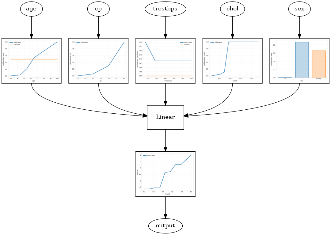
एक टीएफएल डिब्बाबंद आकलनकर्ता का निर्माण करने के लिए, से एक मॉडल विन्यास का निर्माण tfl.configs । एक कैलिब्रेटेड रेखीय मॉडल का उपयोग कर निर्माण किया है tfl.configs.CalibratedLinearConfig । यह इनपुट सुविधाओं पर टुकड़ावार-रैखिक और श्रेणीबद्ध अंशांकन लागू करता है, इसके बाद एक रैखिक संयोजन और एक वैकल्पिक आउटपुट टुकड़ावार-रैखिक अंशांकन होता है। आउटपुट कैलिब्रेशन का उपयोग करते समय या जब आउटपुट सीमाएं निर्दिष्ट की जाती हैं, तो रैखिक परत कैलिब्रेटेड इनपुट पर भारित औसत लागू करेगी।
यह उदाहरण पहली 5 विशेषताओं पर एक कैलिब्रेटेड रैखिक मॉडल बनाता है। हम का उपयोग tfl.visualization अंशशोधक भूखंडों के साथ मॉडल लेखाचित्र तैयार करने।
# Model config defines the model structure for the estimator.
model_config = tfl.configs.CalibratedLinearConfig(
    feature_configs=feature_configs,
    use_bias=True,
    output_calibration=True,
    regularizer_configs=[
        # Regularizer for the output calibrator.
        tfl.configs.RegularizerConfig(name='output_calib_hessian', l2=1e-4),
    ])
# A CannedClassifier is constructed from the given model config.
estimator = tfl.estimators.CannedClassifier(
    feature_columns=feature_columns[:5],
    model_config=model_config,
    feature_analysis_input_fn=feature_analysis_input_fn,
    optimizer=tf.keras.optimizers.Adam(LEARNING_RATE),
    config=tf.estimator.RunConfig(tf_random_seed=42))
estimator.train(input_fn=train_input_fn)
results = estimator.evaluate(input_fn=test_input_fn)
print('Calibrated linear test AUC: {}'.format(results['auc']))
saved_model_path = estimator.export_saved_model(estimator.model_dir,
                                                serving_input_fn)
model_graph = tfl.estimators.get_model_graph(saved_model_path)
tfl.visualization.draw_model_graph(model_graph)
2021-09-30 20:54:06.660239: E tensorflow/stream_executor/cuda/cuda_driver.cc:271] failed call to cuInit: CUDA_ERROR_NO_DEVICE: no CUDA-capable device is detected
Calibrated linear test AUC: 0.834586501121521
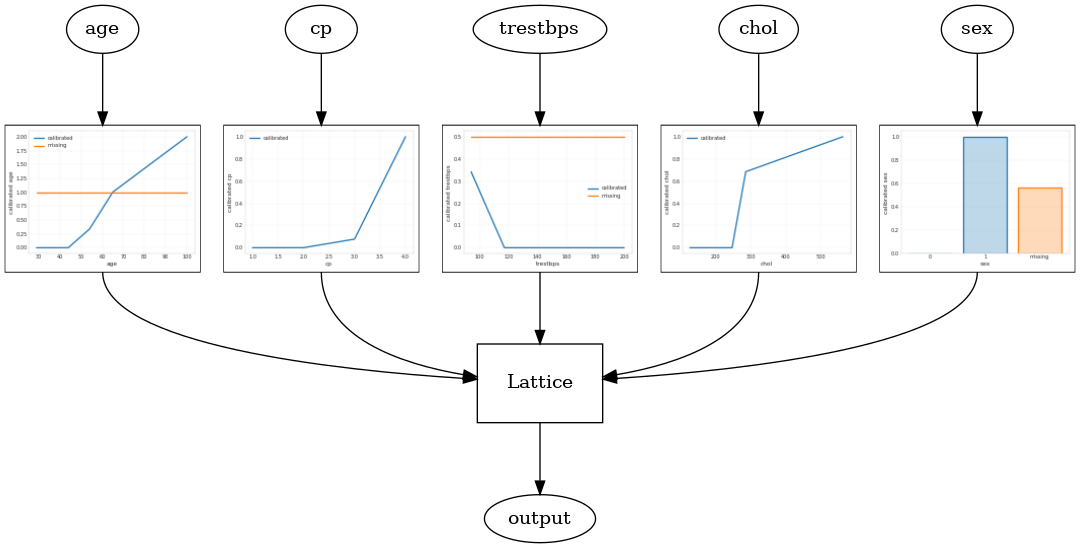
कैलिब्रेटेड जाली मॉडल
एक कैलिब्रेटेड जाली मॉडल का उपयोग कर निर्माण किया है tfl.configs.CalibratedLatticeConfig । एक कैलिब्रेटेड जाली मॉडल इनपुट सुविधाओं पर टुकड़े-टुकड़े-रैखिक और श्रेणीबद्ध अंशांकन लागू करता है, इसके बाद एक जाली मॉडल और एक वैकल्पिक आउटपुट टुकड़ा-रैखिक अंशांकन होता है।
यह उदाहरण पहली 5 विशेषताओं पर एक कैलिब्रेटेड जाली मॉडल बनाता है।
# This is calibrated lattice model: Inputs are calibrated, then combined
# non-linearly using a lattice layer.
model_config = tfl.configs.CalibratedLatticeConfig(
    feature_configs=feature_configs,
    regularizer_configs=[
        # Torsion regularizer applied to the lattice to make it more linear.
        tfl.configs.RegularizerConfig(name='torsion', l2=1e-4),
        # Globally defined calibration regularizer is applied to all features.
        tfl.configs.RegularizerConfig(name='calib_hessian', l2=1e-4),
    ])
# A CannedClassifier is constructed from the given model config.
estimator = tfl.estimators.CannedClassifier(
    feature_columns=feature_columns[:5],
    model_config=model_config,
    feature_analysis_input_fn=feature_analysis_input_fn,
    optimizer=tf.keras.optimizers.Adam(LEARNING_RATE),
    config=tf.estimator.RunConfig(tf_random_seed=42))
estimator.train(input_fn=train_input_fn)
results = estimator.evaluate(input_fn=test_input_fn)
print('Calibrated lattice test AUC: {}'.format(results['auc']))
saved_model_path = estimator.export_saved_model(estimator.model_dir,
                                                serving_input_fn)
model_graph = tfl.estimators.get_model_graph(saved_model_path)
tfl.visualization.draw_model_graph(model_graph)
Calibrated lattice test AUC: 0.8427318930625916
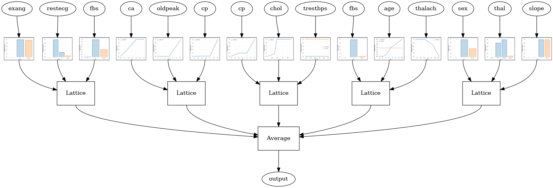
कैलिब्रेटेड जाली एनसेंबल
जब सुविधाओं की संख्या बड़ी होती है, तो आप एक पहनावा मॉडल का उपयोग कर सकते हैं, जो सुविधाओं के सबसेट के लिए कई छोटी जाली बनाता है और केवल एक विशाल जाली बनाने के बजाय उनके आउटपुट को औसत करता है। एनसेंबल जाली मॉडल का उपयोग कर निर्माण कर रहे हैं tfl.configs.CalibratedLatticeEnsembleConfig । एक कैलिब्रेटेड जालीदार पहनावा मॉडल इनपुट फीचर पर टुकड़े-टुकड़े-रैखिक और श्रेणीबद्ध अंशांकन लागू करता है, इसके बाद जाली मॉडल का एक समूह और एक वैकल्पिक आउटपुट टुकड़ा-रैखिक अंशांकन होता है।
यादृच्छिक जाली कलाकारों की टुकड़ी
निम्न मॉडल कॉन्फ़िगरेशन प्रत्येक जाली के लिए सुविधाओं के यादृच्छिक सबसेट का उपयोग करता है।
# This is random lattice ensemble model with separate calibration:
# model output is the average output of separately calibrated lattices.
model_config = tfl.configs.CalibratedLatticeEnsembleConfig(
    feature_configs=feature_configs,
    num_lattices=5,
    lattice_rank=3)
# A CannedClassifier is constructed from the given model config.
estimator = tfl.estimators.CannedClassifier(
    feature_columns=feature_columns,
    model_config=model_config,
    feature_analysis_input_fn=feature_analysis_input_fn,
    optimizer=tf.keras.optimizers.Adam(LEARNING_RATE),
    config=tf.estimator.RunConfig(tf_random_seed=42))
estimator.train(input_fn=train_input_fn)
results = estimator.evaluate(input_fn=test_input_fn)
print('Random ensemble test AUC: {}'.format(results['auc']))
saved_model_path = estimator.export_saved_model(estimator.model_dir,
                                                serving_input_fn)
model_graph = tfl.estimators.get_model_graph(saved_model_path)
tfl.visualization.draw_model_graph(model_graph, calibrator_dpi=15)
Random ensemble test AUC: 0.9003759026527405
RTL परत रैंडम जालीदार पहनावा
निम्नलिखित मॉडल config एक का उपयोग करता है tfl.layers.RTL परत प्रत्येक जाली के लिए सुविधाओं की एक यादृच्छिक सबसेट का उपयोग करता है। हम ध्यान दें कि tfl.layers.RTL केवल दिष्टता की कमी का समर्थन करता है और सभी सुविधाओं के लिए समान जाली आकार और कोई प्रति-सुविधा नियमितीकरण होना आवश्यक है। नोट एक का उपयोग कर कि tfl.layers.RTL परत आप अलग का उपयोग कर से भी ज्यादा बड़ा टुकड़ियों को स्केल की सुविधा देता है tfl.layers.Lattice उदाहरणों।
# Make sure our feature configs have the same lattice size, no per-feature
# regularization, and only monotonicity constraints.
rtl_layer_feature_configs = copy.deepcopy(feature_configs)
for feature_config in rtl_layer_feature_configs:
  feature_config.lattice_size = 2
  feature_config.unimodality = 'none'
  feature_config.reflects_trust_in = None
  feature_config.dominates = None
  feature_config.regularizer_configs = None
# This is RTL layer ensemble model with separate calibration:
# model output is the average output of separately calibrated lattices.
model_config = tfl.configs.CalibratedLatticeEnsembleConfig(
    lattices='rtl_layer',
    feature_configs=rtl_layer_feature_configs,
    num_lattices=5,
    lattice_rank=3)
# A CannedClassifier is constructed from the given model config.
estimator = tfl.estimators.CannedClassifier(
    feature_columns=feature_columns,
    model_config=model_config,
    feature_analysis_input_fn=feature_analysis_input_fn,
    optimizer=tf.keras.optimizers.Adam(LEARNING_RATE),
    config=tf.estimator.RunConfig(tf_random_seed=42))
estimator.train(input_fn=train_input_fn)
results = estimator.evaluate(input_fn=test_input_fn)
print('Random ensemble test AUC: {}'.format(results['auc']))
saved_model_path = estimator.export_saved_model(estimator.model_dir,
                                                serving_input_fn)
model_graph = tfl.estimators.get_model_graph(saved_model_path)
tfl.visualization.draw_model_graph(model_graph, calibrator_dpi=15)
Random ensemble test AUC: 0.8903509378433228
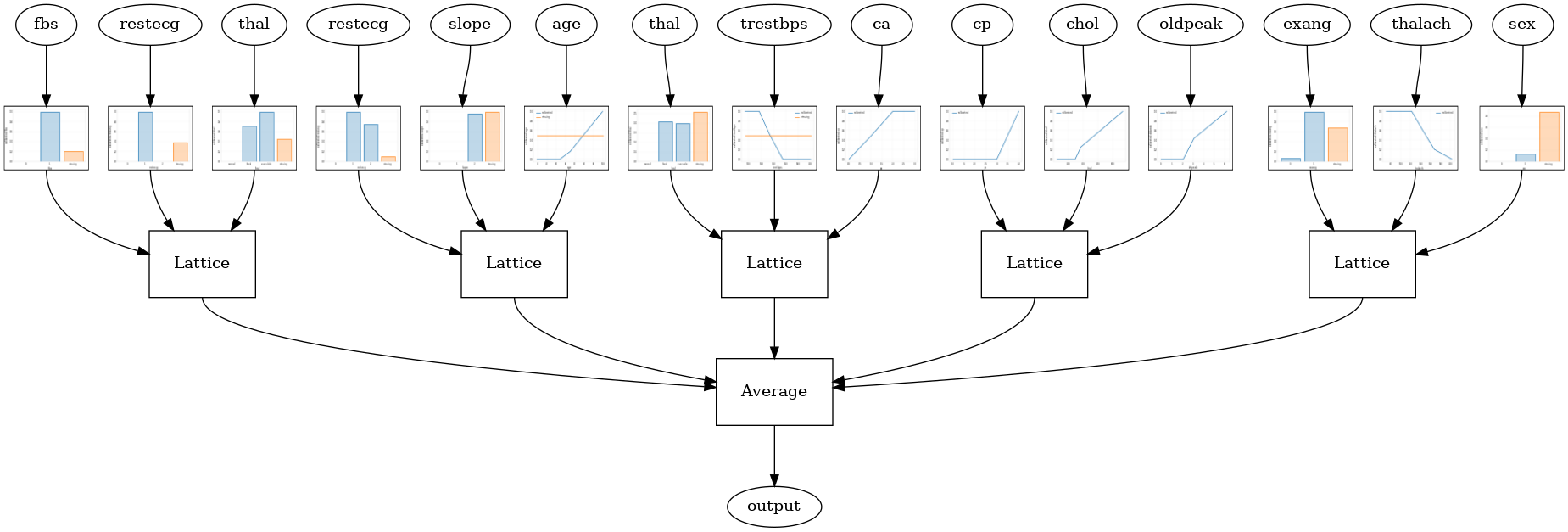
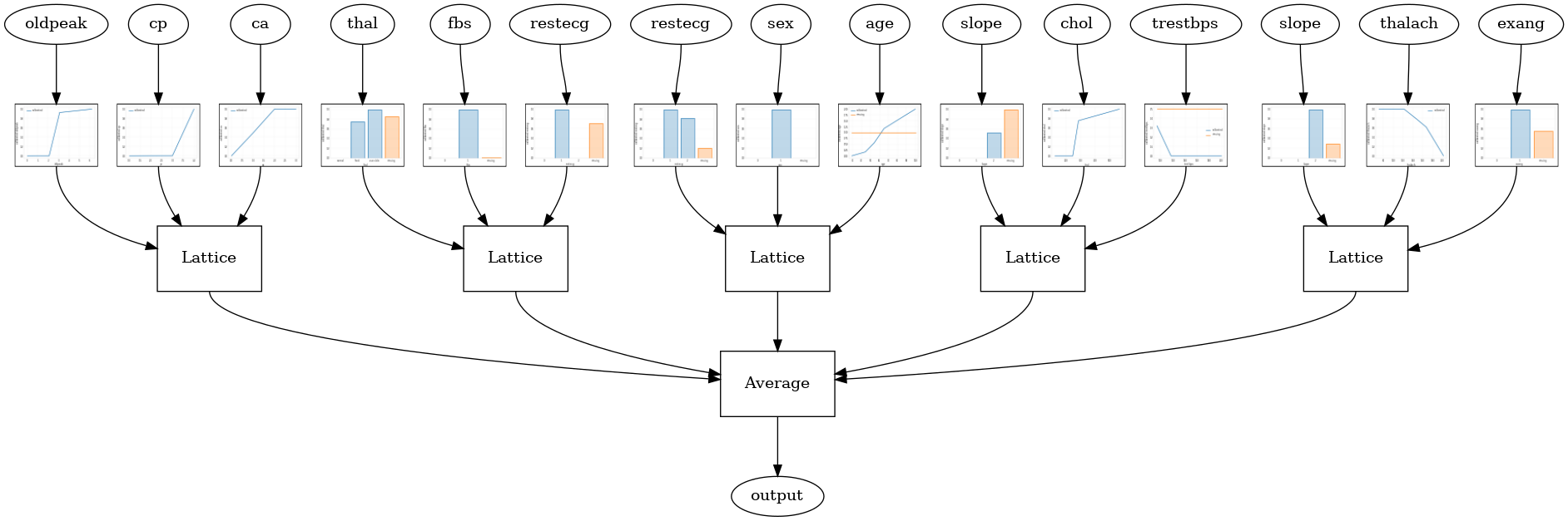
क्रिस्टल जाली पहनावा
टीएफएल भी एक अनुमानी सुविधा व्यवस्था एल्गोरिथ्म, कहा जाता है प्रदान करता है कण । कण पहले गाड़ियों एल्गोरिथ्म एक prefitting मॉडल है कि अनुमान सुविधा बातचीत जोड़ो में। यह तब अंतिम पहनावा की व्यवस्था करता है जैसे कि अधिक गैर-रैखिक इंटरैक्शन वाली विशेषताएं एक ही जाली में हों।
क्रिस्टल मॉडल के लिए, आप भी एक प्रदान करना होगा prefitting_input_fn जैसा कि ऊपर वर्णित है कि, prefitting मॉडल प्रशिक्षित करने के लिए प्रयोग किया जाता है। प्रीफिटिंग मॉडल को पूरी तरह से प्रशिक्षित होने की आवश्यकता नहीं है, इसलिए कुछ युग पर्याप्त होने चाहिए।
prefitting_input_fn = tf.compat.v1.estimator.inputs.pandas_input_fn(
    x=train_x,
    y=train_y,
    shuffle=False,
    batch_size=BATCH_SIZE,
    num_epochs=PREFITTING_NUM_EPOCHS,
    num_threads=1)
इसके बाद आप स्थापना करके एक क्रिस्टल मॉडल बना सकते हैं lattice='crystals' मॉडल config में।
# This is Crystals ensemble model with separate calibration: model output is
# the average output of separately calibrated lattices.
model_config = tfl.configs.CalibratedLatticeEnsembleConfig(
    feature_configs=feature_configs,
    lattices='crystals',
    num_lattices=5,
    lattice_rank=3)
# A CannedClassifier is constructed from the given model config.
estimator = tfl.estimators.CannedClassifier(
    feature_columns=feature_columns,
    model_config=model_config,
    feature_analysis_input_fn=feature_analysis_input_fn,
    # prefitting_input_fn is required to train the prefitting model.
    prefitting_input_fn=prefitting_input_fn,
    optimizer=tf.keras.optimizers.Adam(LEARNING_RATE),
    prefitting_optimizer=tf.keras.optimizers.Adam(LEARNING_RATE),
    config=tf.estimator.RunConfig(tf_random_seed=42))
estimator.train(input_fn=train_input_fn)
results = estimator.evaluate(input_fn=test_input_fn)
print('Crystals ensemble test AUC: {}'.format(results['auc']))
saved_model_path = estimator.export_saved_model(estimator.model_dir,
                                                serving_input_fn)
model_graph = tfl.estimators.get_model_graph(saved_model_path)
tfl.visualization.draw_model_graph(model_graph, calibrator_dpi=15)
Crystals ensemble test AUC: 0.8840851783752441
आप का उपयोग कर अधिक विवरण के साथ सुविधा calibrators प्लॉट कर सकते हैं tfl.visualization मॉड्यूल।
_ = tfl.visualization.plot_feature_calibrator(model_graph, "age")
_ = tfl.visualization.plot_feature_calibrator(model_graph, "restecg")

