
| | |  GitHub-এ উৎস দেখুন GitHub-এ উৎস দেখুন | |
এই কোল্যাবে, আমরা টেনসরফ্লো এবং টেনসরফ্লো সম্ভাব্যতা ব্যবহার করে গাউসিয়ান প্রসেস রিগ্রেশন অন্বেষণ করি। আমরা কিছু পরিচিত ফাংশন থেকে কিছু শোরগোল পর্যবেক্ষন তৈরি করি এবং সেই ডেটাতে জিপি মডেলগুলিকে ফিট করি। তারপরে আমরা জিপি পোস্টেরিয়র থেকে নমুনা করি এবং তাদের ডোমেনে গ্রিডের উপর নমুনাযুক্ত ফাংশন মানগুলি প্লট করি।
পটভূমি
যাক \(\mathcal{X}\) কোনও হতে। একজন গসিয়ান প্রক্রিয়া (জিপি) দ্বারা সূচীবদ্ধ র্যান্ডম ভেরিয়েবল একটি সংগ্রহ \(\mathcal{X}\) যেমন যে যদি\(\{X_1, \ldots, X_n\} \subset \mathcal{X}\) কোন সসীম উপসেট হয়, প্রান্তিক ঘনত্ব\(p(X_1 = x_1, \ldots, X_n = x_n)\) বহুচলকীয় হয় গসিয়ান। যেকোন গাউসিয়ান ডিস্ট্রিবিউশন সম্পূর্ণরূপে তার প্রথম এবং দ্বিতীয় কেন্দ্রীয় মুহূর্ত (গড় এবং কোভেরিয়েন্স) দ্বারা নির্দিষ্ট করা হয়, এবং GP এর ব্যতিক্রম নয়। আমরা তার গড় ফাংশন পরিপ্রেক্ষিতে সম্পূর্ণ জিপি নির্দিষ্ট করতে পারেন \(\mu : \mathcal{X} \to \mathbb{R}\) এবং সহভেদাংক ফাংশন\(k : \mathcal{X} \times \mathcal{X} \to \mathbb{R}\)। জিপি-এর বেশিরভাগ অভিব্যক্তিমূলক শক্তি কোভেরিয়েন্স ফাংশনের পছন্দের মধ্যে আবদ্ধ। বিভিন্ন কারণে, সহভেদাংক ফাংশন একটি কার্নেল ফাংশন হিসাবে উল্লেখ করা হয়। এটা শুধুমাত্র প্রতিসম এবং ইতিবাচক-নির্দিষ্ট হতে (দেখুন প্রয়োজন বোধ করা হয় অধ্যায়। রাসমুসেন ও উইলিয়ামস 4 )। নীচে আমরা Exponentiated Quadratic covariance কার্নেল ব্যবহার করি। এর রূপ হল
\[ k(x, x') := \sigma^2 \exp \left( \frac{\|x - x'\|^2}{\lambda^2} \right) \]
যেখানে \(\sigma^2\) 'প্রশস্ততা' এবং বলা হয় \(\lambda\) দৈর্ঘ্য স্কেল। কার্নেল পরামিতিগুলি সর্বাধিক সম্ভাবনা অপ্টিমাইজেশন পদ্ধতির মাধ্যমে নির্বাচন করা যেতে পারে।
একটি জিপি থেকে একটি পূর্ণ নমুনা সমগ্র স্থান উপর একটি বাস্তব-মান ফাংশন গঠিত\(\mathcal{X}\) ও অনুশীলন বুঝতে অকার্যকর হয়; প্রায়শই কেউ একটি নমুনা পর্যবেক্ষণ করার জন্য পয়েন্টগুলির একটি সেট বেছে নেয় এবং এই পয়েন্টগুলিতে ফাংশনের মান আঁকে। এটি একটি উপযুক্ত (সসীম-মাত্রিক) বহু-ভেরিয়েট গাউসিয়ান থেকে নমুনা দ্বারা অর্জন করা হয়।
উল্লেখ্য যে, উপরোক্ত সংজ্ঞা অনুসারে, যেকোন সসীম-মাত্রিক মাল্টিভেরিয়েট গাউসিয়ান ডিস্ট্রিবিউশনও একটি গাউসিয়ান প্রক্রিয়া। সাধারণত, যখন এক একটি জিপি বোঝায়, এটা অন্তর্নিহিত যে সূচক সেট কিছু হয় \(\mathbb{R}^n\)এবং আমরা অবশ্যই এখানে এই ধৃষ্টতা করতে হবে।
মেশিন লার্নিংয়ে গাউসিয়ান প্রক্রিয়ার একটি সাধারণ প্রয়োগ হল গাউসিয়ান প্রক্রিয়া রিগ্রেশন। ধারণা যে আমরা একটি অজানা ফাংশন দেওয়া সশব্দ পর্যবেক্ষণ অনুমান করতে ইচ্ছুক \(\{y_1, \ldots, y_N\}\) পয়েন্ট একটি নির্দিষ্ট নম্বরে ফাংশনের \(\{x_1, \ldots x_N\}.\) আমরা একটি সৃজক প্রক্রিয়া কল্পনা
\[ \begin{align} f \sim \: & \textsf{GaussianProcess}\left( \text{mean_fn}=\mu(x), \text{covariance_fn}=k(x, x')\right) \\ y_i \sim \: & \textsf{Normal}\left( \text{loc}=f(x_i), \text{scale}=\sigma\right), i = 1, \ldots, N \end{align} \]
উপরে উল্লিখিত হিসাবে, নমুনাকৃত ফাংশন গণনা করা অসম্ভব, যেহেতু আমাদের একটি অসীম সংখ্যক পয়েন্টে এর মান প্রয়োজন। পরিবর্তে, কেউ একটি মাল্টিভেরিয়েট গাউসিয়ান থেকে একটি সীমিত নমুনা বিবেচনা করে।
\[ \begin{gather} \begin{bmatrix} f(x_1) \\ \vdots \\ f(x_N) \end{bmatrix} \sim \textsf{MultivariateNormal} \left( \: \text{loc}= \begin{bmatrix} \mu(x_1) \\ \vdots \\ \mu(x_N) \end{bmatrix} \:,\: \text{scale}= \begin{bmatrix} k(x_1, x_1) & \cdots & k(x_1, x_N) \\ \vdots & \ddots & \vdots \\ k(x_N, x_1) & \cdots & k(x_N, x_N) \\ \end{bmatrix}^{1/2} \: \right) \end{gather} \\ y_i \sim \textsf{Normal} \left( \text{loc}=f(x_i), \text{scale}=\sigma \right) \]
উল্লেখ্য এক্সপোনেন্ট \(\frac{1}{2}\) সহভেদাংক ম্যাট্রিক্স করুন: এই একটি Cholesky পচানি উল্লেখ করে। কোলেস্কি কম্পিউট করা প্রয়োজন কারণ MVN হল একটি অবস্থান-স্কেল পারিবারিক বিতরণ। দুর্ভাগ্যবশত Cholesky পচানি গণনা ব্যয়বহুল, গ্রহণ \(O(N^3)\) সময় এবং \(O(N^2)\) স্থান। জিপি সাহিত্যের বেশিরভাগই এই আপাতদৃষ্টিতে নিরীহ সামান্য ব্যাখ্যাকারীর সাথে মোকাবিলা করার উপর দৃষ্টি নিবদ্ধ করে।
পূর্বের গড় ফাংশনটিকে ধ্রুবক, প্রায়শই শূন্য হিসাবে নেওয়া সাধারণ। এছাড়াও, কিছু নোটেশনাল কনভেনশন সুবিধাজনক। এক প্রায়ই লিখেছেন \(\mathbf{f}\) নমুনা ফাংশন মূল্যবোধের সসীম ভেক্টর জন্য। আকর্ষণীয় স্বরলিপি বেশ কয়েকটি সহভেদাংক ম্যাট্রিক্স প্রয়োগ ফলে জন্য ব্যবহার করা হয় \(k\) ইনপুট জোড়া জন্য। অনুসরণ করছেন (Quiñonero-Candela, 2005) , আমরা লক্ষ করুন যে, ম্যাট্রিক্সের উপাদান বিশেষ ইনপুট বিন্দুতে ফাংশন মূল্যবোধের covariances হয়। সুতরাং আমরা সহভেদাংক ম্যাট্রিক্স বোঝাতে পারে \(K_{AB}\)যেখানে \(A\) এবং \(B\) দেওয়া ম্যাট্রিক্স মাত্রা বরাবর ফাংশন মূল্যবোধের সংগ্রহে কিছু সূচক।
উদাহরণস্বরূপ, প্রদত্ত পর্যবেক্ষিত তথ্য \((\mathbf{x}, \mathbf{y})\) উহ্য সুপ্ত ফাংশন মান \(\mathbf{f}\), আমরা লিখতে পারি
\[ K_{\mathbf{f},\mathbf{f} } = \begin{bmatrix} k(x_1, x_1) & \cdots & k(x_1, x_N) \\ \vdots & \ddots & \vdots \\ k(x_N, x_1) & \cdots & k(x_N, x_N) \\ \end{bmatrix} \]
একইভাবে, আমরা ইনপুট সেট মিশ্রিত করতে পারেন, যেমন
\[ K_{\mathbf{f},*} = \begin{bmatrix} k(x_1, x^*_1) & \cdots & k(x_1, x^*_T) \\ \vdots & \ddots & \vdots \\ k(x_N, x^*_1) & \cdots & k(x_N, x^*_T) \\ \end{bmatrix} \]
যেখানে আমরা অনুমান করা আছে \(N\) প্রশিক্ষণ ইনপুট, এবং \(T\) পরীক্ষা ইনপুট। উপরে উত্পাদিত প্রক্রিয়া তারপর কম্প্যাক্টলি হিসাবে লিখিত হতে পারে
\[ \begin{align} \mathbf{f} \sim \: & \textsf{MultivariateNormal} \left( \text{loc}=\mathbf{0}, \text{scale}=K_{\mathbf{f},\mathbf{f} }^{1/2} \right) \\ y_i \sim \: & \textsf{Normal} \left( \text{loc}=f_i, \text{scale}=\sigma \right), i = 1, \ldots, N \end{align} \]
প্রথম লাইনে স্যাম্পলিং অপারেশন একটি নির্দিষ্ট সেট উৎপাদ \(N\) না স্বরলিপি জিপি উপরে আঁকা হিসেবে একটি সম্পূর্ণ ফাংশন - একটি বহুচলকীয় গসিয়ান থেকে ফাংশন মান। দ্বিতীয় লাইন একটি সংগ্রহ বর্ণনা করে \(N\) স্বপক্ষে থেকে univariate Gaussians বিভিন্ন ফাংশন মান কেন্দ্রীভূত, স্থায়ী পর্যবেক্ষণ গোলমাল সঙ্গে \(\sigma^2\)।
উপরের জেনারেটিভ মডেলের জায়গায়, আমরা পোস্টেরিয়র ইনফারেন্স সমস্যা বিবেচনা করতে এগিয়ে যেতে পারি। এটি পরীক্ষা পয়েন্টের একটি নতুন সেটে ফাংশন মানগুলির উপর একটি পশ্চাৎবর্তী বন্টন দেয়, উপরের প্রক্রিয়া থেকে পর্যবেক্ষণ করা গোলমাল ডেটার উপর শর্তযুক্ত।
জায়গায় উপরে স্বরলিপি সঙ্গে, আমরা কষে ভবিষ্যত নিয়ে অবর ভবিষ্যদ্বাণীপূর্ণ বন্টন লিখতে পারেন (সশব্দ) পর্যবেক্ষণ সংশ্লিষ্ট ইনপুট ও প্রশিক্ষণ তথ্য হিসাবে অনুসরণ করে (আরো বিস্তারিত জানার জন্য, এর §2.2 দেখেন শর্তসাপেক্ষ রাসমুসেন ও উইলিয়ামস )।
\[ \mathbf{y}^* \mid \mathbf{x}^*, \mathbf{x}, \mathbf{y} \sim \textsf{Normal} \left( \text{loc}=\mathbf{\mu}^*, \text{scale}=(\Sigma^*)^{1/2} \right), \]
কোথায়
\[ \mathbf{\mu}^* = K_{*,\mathbf{f} }\left(K_{\mathbf{f},\mathbf{f} } + \sigma^2 I \right)^{-1} \mathbf{y} \]
এবং
\[ \Sigma^* = K_{*,*} - K_{*,\mathbf{f} } \left(K_{\mathbf{f},\mathbf{f} } + \sigma^2 I \right)^{-1} K_{\mathbf{f},*} \]
আমদানি
import time

import numpy as np
import matplotlib.pyplot as plt
import tensorflow.compat.v2 as tf
import tensorflow_probability as tfp
tfb = tfp.bijectors
tfd = tfp.distributions
tfk = tfp.math.psd_kernels
tf.enable_v2_behavior()

from mpl_toolkits.mplot3d import Axes3D
%pylab inline
# Configure plot defaults
plt.rcParams['axes.facecolor'] = 'white'
plt.rcParams['grid.color'] = '#666666'
%config InlineBackend.figure_format = 'png'
Populating the interactive namespace from numpy and matplotlib
উদাহরণ: শোরগোল সাইনুসয়েডাল ডেটাতে সঠিক জিপি রিগ্রেশন
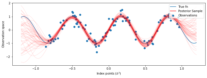
এখানে আমরা একটি কোলাহলপূর্ণ সাইনুসয়েড থেকে প্রশিক্ষণের ডেটা তৈরি করি, তারপর জিপি রিগ্রেশন মডেলের পশ্চাৎভাগ থেকে বক্ররেখার একটি গুচ্ছ নমুনা করি। আমরা ব্যবহার আদম কার্নেল hyperparameters (আমরা পূর্বে অধীনে ডেটার নেতিবাচক লগ সম্ভাবনা কমান) নিখুত। আমরা প্রশিক্ষণ বক্ররেখা প্লট করি, তারপরে সত্যিকারের ফাংশন এবং পশ্চাদবর্তী নমুনাগুলি অনুসরণ করি।
def sinusoid(x):
  return np.sin(3 * np.pi * x[..., 0])

def generate_1d_data(num_training_points, observation_noise_variance):
  """Generate noisy sinusoidal observations at a random set of points.

  Returns:
     observation_index_points, observations
  """
  index_points_ = np.random.uniform(-1., 1., (num_training_points, 1))
  index_points_ = index_points_.astype(np.float64)
  # y = f(x) + noise
  observations_ = (sinusoid(index_points_) +
                   np.random.normal(loc=0,
                                    scale=np.sqrt(observation_noise_variance),
                                    size=(num_training_points)))
  return index_points_, observations_
# Generate training data with a known noise level (we'll later try to recover
# this value from the data).
NUM_TRAINING_POINTS = 100
observation_index_points_, observations_ = generate_1d_data(
    num_training_points=NUM_TRAINING_POINTS,
    observation_noise_variance=.1)
আমরা কার্নেল hyperparameters উপর গতকাল দেশের সর্বোচ্চ তাপমাত্রা করা, এবং hyperparameters এবং পর্যবেক্ষিত ডেটা ব্যবহার যুগ্ম বিতরণ লিখবো tfd.JointDistributionNamed ।
def build_gp(amplitude, length_scale, observation_noise_variance):
  """Defines the conditional dist. of GP outputs, given kernel parameters."""

  # Create the covariance kernel, which will be shared between the prior (which we
  # use for maximum likelihood training) and the posterior (which we use for
  # posterior predictive sampling)
  kernel = tfk.ExponentiatedQuadratic(amplitude, length_scale)

  # Create the GP prior distribution, which we will use to train the model
  # parameters.
  return tfd.GaussianProcess(
      kernel=kernel,
      index_points=observation_index_points_,
      observation_noise_variance=observation_noise_variance)

gp_joint_model = tfd.JointDistributionNamed({
    'amplitude': tfd.LogNormal(loc=0., scale=np.float64(1.)),
    'length_scale': tfd.LogNormal(loc=0., scale=np.float64(1.)),
    'observation_noise_variance': tfd.LogNormal(loc=0., scale=np.float64(1.)),
    'observations': build_gp,
})
আমরা আগে থেকে নমুনা নিতে পারি এবং একটি নমুনার লগ-ঘনত্ব গণনা করতে পারি তা যাচাই করে আমরা আমাদের বাস্তবায়ন পরীক্ষা করতে পারি।
x = gp_joint_model.sample()
lp = gp_joint_model.log_prob(x)

print("sampled {}".format(x))
print("log_prob of sample: {}".format(lp))
sampled {'observation_noise_variance': <tf.Tensor: shape=(), dtype=float64, numpy=2.067952217184325>, 'length_scale': <tf.Tensor: shape=(), dtype=float64, numpy=1.154435715487831>, 'amplitude': <tf.Tensor: shape=(), dtype=float64, numpy=5.383850737703549>, 'observations': <tf.Tensor: shape=(100,), dtype=float64, numpy=
array([-2.37070577, -2.05363838, -0.95152824,  3.73509388, -0.2912646 ,
        0.46112342, -1.98018513, -2.10295857, -1.33589756, -2.23027226,
       -2.25081374, -0.89450835, -2.54196452,  1.46621647,  2.32016193,
        5.82399989,  2.27241034, -0.67523432, -1.89150197, -1.39834474,
       -2.33954116,  0.7785609 , -1.42763627, -0.57389025, -0.18226098,
       -3.45098732,  0.27986652, -3.64532398, -1.28635204, -2.42362875,
        0.01107288, -2.53222176, -2.0886136 , -5.54047694, -2.18389607,
       -1.11665628, -3.07161217, -2.06070336, -0.84464262,  1.29238438,
       -0.64973999, -2.63805504, -3.93317576,  0.65546645,  2.24721181,
       -0.73403676,  5.31628298, -1.2208384 ,  4.77782252, -1.42978168,
       -3.3089274 ,  3.25370494,  3.02117591, -1.54862932, -1.07360811,
        1.2004856 , -4.3017773 , -4.95787789, -1.95245901, -2.15960839,
       -3.78592731, -1.74096185,  3.54891595,  0.56294143,  1.15288455,
       -0.77323696,  2.34430694, -1.05302007, -0.7514684 , -0.98321063,
       -3.01300144, -3.00033274,  0.44200837,  0.45060886, -1.84497318,
       -1.89616746, -2.15647664, -2.65672581, -3.65493379,  1.70923375,
       -3.88695218, -0.05151283,  4.51906677, -2.28117003,  3.03032793,
       -1.47713194, -0.35625273,  3.73501587, -2.09328047, -0.60665614,
       -0.78177188, -0.67298545,  2.97436033, -0.29407932,  2.98482427,
       -1.54951178,  2.79206821,  4.2225733 ,  2.56265198,  2.80373284])>}
log_prob of sample: -194.96442183797524
এখন সর্বোচ্চ পোস্টেরিয়র সম্ভাব্যতা সহ পরামিতি মান খুঁজে পেতে অপ্টিমাইজ করা যাক। আমরা প্রতিটি প্যারামিটারের জন্য একটি পরিবর্তনশীল সংজ্ঞায়িত করব এবং তাদের মানকে ইতিবাচক হতে সীমাবদ্ধ করব।
# Create the trainable model parameters, which we'll subsequently optimize.
# Note that we constrain them to be strictly positive.

constrain_positive = tfb.Shift(np.finfo(np.float64).tiny)(tfb.Exp())

amplitude_var = tfp.util.TransformedVariable(
    initial_value=1.,
    bijector=constrain_positive,
    name='amplitude',
    dtype=np.float64)

length_scale_var = tfp.util.TransformedVariable(
    initial_value=1.,
    bijector=constrain_positive,
    name='length_scale',
    dtype=np.float64)

observation_noise_variance_var = tfp.util.TransformedVariable(
    initial_value=1.,
    bijector=constrain_positive,
    name='observation_noise_variance_var',
    dtype=np.float64)

trainable_variables = [v.trainable_variables[0] for v in
                       [amplitude_var,
                       length_scale_var,
                       observation_noise_variance_var]]
আমাদের পর্যবেক্ষিত ডেটার উপর মডেল অবস্থা, আমরা একটি সংজ্ঞায়িত করব target_log_prob ফাংশন, যা (এখনও অনুমান করা পর্যন্ত) কার্নেল hyperparameters লাগে।
def target_log_prob(amplitude, length_scale, observation_noise_variance):
  return gp_joint_model.log_prob({
      'amplitude': amplitude,
      'length_scale': length_scale,
      'observation_noise_variance': observation_noise_variance,
      'observations': observations_
  })
# Now we optimize the model parameters.
num_iters = 1000
optimizer = tf.optimizers.Adam(learning_rate=.01)

# Use `tf.function` to trace the loss for more efficient evaluation.
@tf.function(autograph=False, jit_compile=False)
def train_model():
  with tf.GradientTape() as tape:
    loss = -target_log_prob(amplitude_var, length_scale_var,
                            observation_noise_variance_var)
  grads = tape.gradient(loss, trainable_variables)
  optimizer.apply_gradients(zip(grads, trainable_variables))
  return loss

# Store the likelihood values during training, so we can plot the progress
lls_ = np.zeros(num_iters, np.float64)
for i in range(num_iters):
  loss = train_model()
  lls_[i] = loss

print('Trained parameters:')
print('amplitude: {}'.format(amplitude_var._value().numpy()))
print('length_scale: {}'.format(length_scale_var._value().numpy()))
print('observation_noise_variance: {}'.format(observation_noise_variance_var._value().numpy()))
Trained parameters:
amplitude: 0.9176153445125278
length_scale: 0.18444082442910079
observation_noise_variance: 0.0880273312850989
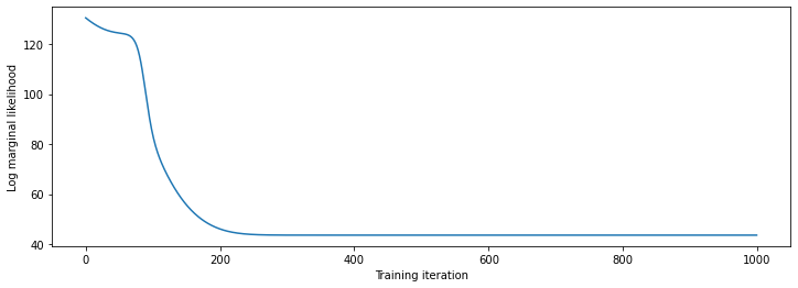
# Plot the loss evolution
plt.figure(figsize=(12, 4))
plt.plot(lls_)
plt.xlabel("Training iteration")
plt.ylabel("Log marginal likelihood")
plt.show()
# Having trained the model, we'd like to sample from the posterior conditioned
# on observations. We'd like the samples to be at points other than the training
# inputs.
predictive_index_points_ = np.linspace(-1.2, 1.2, 200, dtype=np.float64)
# Reshape to [200, 1] -- 1 is the dimensionality of the feature space.
predictive_index_points_ = predictive_index_points_[..., np.newaxis]

optimized_kernel = tfk.ExponentiatedQuadratic(amplitude_var, length_scale_var)
gprm = tfd.GaussianProcessRegressionModel(
    kernel=optimized_kernel,
    index_points=predictive_index_points_,
    observation_index_points=observation_index_points_,
    observations=observations_,
    observation_noise_variance=observation_noise_variance_var,
    predictive_noise_variance=0.)

# Create op to draw  50 independent samples, each of which is a *joint* draw
# from the posterior at the predictive_index_points_. Since we have 200 input
# locations as defined above, this posterior distribution over corresponding
# function values is a 200-dimensional multivariate Gaussian distribution!
num_samples = 50
samples = gprm.sample(num_samples)
# Plot the true function, observations, and posterior samples.
plt.figure(figsize=(12, 4))
plt.plot(predictive_index_points_, sinusoid(predictive_index_points_),
         label='True fn')
plt.scatter(observation_index_points_[:, 0], observations_,
            label='Observations')
for i in range(num_samples):
  plt.plot(predictive_index_points_, samples[i, :], c='r', alpha=.1,
           label='Posterior Sample' if i == 0 else None)
leg = plt.legend(loc='upper right')
for lh in leg.legendHandles:
    lh.set_alpha(1)
plt.xlabel(r"Index points ($\mathbb{R}^1$)")
plt.ylabel("Observation space")
plt.show()
HMC সহ প্রান্তিক হাইপারপ্যারামিটার
হাইপারপ্যারামিটারগুলি অপ্টিমাইজ করার পরিবর্তে, হ্যামিলটোনিয়ান মন্টে কার্লোর সাথে সেগুলিকে একীভূত করার চেষ্টা করা যাক। আমরা প্রথমে একটি স্যাম্পলারকে সংজ্ঞায়িত করব এবং চালনা করব যাতে কার্নেল হাইপারপ্যারামিটারের উপর পোস্টেরিয়র ডিস্ট্রিবিউশন থেকে আনুমানিকভাবে আঁকতে হয়।
num_results = 100
num_burnin_steps = 50

sampler = tfp.mcmc.TransformedTransitionKernel(
    tfp.mcmc.NoUTurnSampler(
        target_log_prob_fn=target_log_prob,
        step_size=tf.cast(0.1, tf.float64)),
    bijector=[constrain_positive, constrain_positive, constrain_positive])

adaptive_sampler = tfp.mcmc.DualAveragingStepSizeAdaptation(
    inner_kernel=sampler,
    num_adaptation_steps=int(0.8 * num_burnin_steps),
    target_accept_prob=tf.cast(0.75, tf.float64))

initial_state = [tf.cast(x, tf.float64) for x in [1., 1., 1.]]
# Speed up sampling by tracing with `tf.function`.
@tf.function(autograph=False, jit_compile=False)
def do_sampling():
  return tfp.mcmc.sample_chain(
      kernel=adaptive_sampler,
      current_state=initial_state,
      num_results=num_results,
      num_burnin_steps=num_burnin_steps,
      trace_fn=lambda current_state, kernel_results: kernel_results)

t0 = time.time()
samples, kernel_results = do_sampling()
t1 = time.time()
print("Inference ran in {:.2f}s.".format(t1-t0))
Inference ran in 9.00s.
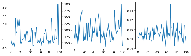
আসুন হাইপারপ্যারামিটার ট্রেসগুলি পরীক্ষা করে স্যানিটি-চেক করি।
(amplitude_samples,
 length_scale_samples,
 observation_noise_variance_samples) = samples

f = plt.figure(figsize=[15, 3])
for i, s in enumerate(samples):
  ax = f.add_subplot(1, len(samples) + 1, i + 1)
  ax.plot(s)
এখন পরিবর্তে অপ্টিমাইজ hyperparameters সঙ্গে একটি একক জিপি নির্মানের, আমরা GPS -এর একটি মিশ্রণ, প্রতিটি hyperparameters উপর অবর বন্টন থেকে একটি নমুনা দ্বারা সংজ্ঞায়িত হিসাবে অবর ভবিষ্যদ্বাণীপূর্ণ বন্টন গঠন করা। এটি আনুমানিকভাবে মন্টে কার্লো স্যাম্পলিংয়ের মাধ্যমে পশ্চাৎপদ পরামিতিগুলির উপর একীভূত করে অপ্রদর্শিত অবস্থানে প্রান্তিক ভবিষ্যদ্বাণীমূলক বিতরণ গণনা করতে।
# The sampled hyperparams have a leading batch dimension, `[num_results, ...]`,
# so they construct a *batch* of kernels.
batch_of_posterior_kernels = tfk.ExponentiatedQuadratic(
    amplitude_samples, length_scale_samples)

# The batch of kernels creates a batch of GP predictive models, one for each
# posterior sample.
batch_gprm = tfd.GaussianProcessRegressionModel(
    kernel=batch_of_posterior_kernels,
    index_points=predictive_index_points_,
    observation_index_points=observation_index_points_,
    observations=observations_,
    observation_noise_variance=observation_noise_variance_samples,
    predictive_noise_variance=0.)

# To construct the marginal predictive distribution, we average with uniform
# weight over the posterior samples.
predictive_gprm = tfd.MixtureSameFamily(
    mixture_distribution=tfd.Categorical(logits=tf.zeros([num_results])),
    components_distribution=batch_gprm)

num_samples = 50
samples = predictive_gprm.sample(num_samples)
# Plot the true function, observations, and posterior samples.
plt.figure(figsize=(12, 4))
plt.plot(predictive_index_points_, sinusoid(predictive_index_points_),
         label='True fn')
plt.scatter(observation_index_points_[:, 0], observations_,
            label='Observations')
for i in range(num_samples):
  plt.plot(predictive_index_points_, samples[i, :], c='r', alpha=.1,
           label='Posterior Sample' if i == 0 else None)
leg = plt.legend(loc='upper right')
for lh in leg.legendHandles:
    lh.set_alpha(1)
plt.xlabel(r"Index points ($\mathbb{R}^1$)")
plt.ylabel("Observation space")
plt.show()
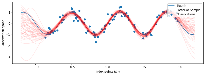
যদিও এই ক্ষেত্রে পার্থক্যগুলি সূক্ষ্ম, সাধারণভাবে, আমরা আশা করব যে আমরা উপরের মতো সম্ভাব্য প্যারামিটারগুলি ব্যবহার করার চেয়ে পোস্টেরিয়র ভবিষ্যদ্বাণীমূলক বন্টনটি আরও ভাল সাধারণীকরণ করবে (ডেটা ধরে রাখার উচ্চ সম্ভাবনা দেবে)।