| | |  Visualizza la fonte su GitHub Visualizza la fonte su GitHub |
JointDistributionSequential è una distribuzione simile a Class di nuova introduzione che consente agli utenti di veloce del prototipo del modello bayesiano. Ti consente di concatenare più distribuzioni e utilizzare la funzione lambda per introdurre dipendenze. Questo è progettato per costruire modelli bayesiani di piccole e medie dimensioni, inclusi molti modelli comunemente usati come GLM, modelli a effetti misti, modelli misti e altro ancora. Abilita tutte le funzionalità necessarie per un flusso di lavoro bayesiano: campionamento predittivo precedente, potrebbe essere collegato a un altro modello grafico bayesiano o rete neurale più grande. In questo Colab, vi mostreremo alcuni esempi di come utilizzare JointDistributionSequential per raggiungere il vostro giorno per giorno il flusso di lavoro bayesiano
Dipendenze e prerequisiti
# We will be using ArviZ, a multi-backend Bayesian diagnosis and plotting librarypip3 install -q git+git://github.com/arviz-devs/arviz.git
Importa e configura
from pprint import pprint
import matplotlib.pyplot as plt
import numpy as np
import seaborn as sns
import pandas as pd
import arviz as az

import tensorflow.compat.v2 as tf
tf.enable_v2_behavior()

import tensorflow_probability as tfp

sns.reset_defaults()
#sns.set_style('whitegrid')
#sns.set_context('talk')
sns.set_context(context='talk',font_scale=0.7)

%config InlineBackend.figure_format = 'retina'
%matplotlib inline

tfd = tfp.distributions
tfb = tfp.bijectors

dtype = tf.float64
Fai le cose velocemente!
Prima di immergerci, assicuriamoci di utilizzare una GPU per questa demo.
Per fare ciò, seleziona "Runtime" -> "Cambia tipo di runtime" -> "Acceleratore hardware" -> "GPU".
Il seguente frammento verificherà che abbiamo accesso a una GPU.
if tf.test.gpu_device_name() != '/device:GPU:0':
  print('WARNING: GPU device not found.')
else:
  print('SUCCESS: Found GPU: {}'.format(tf.test.gpu_device_name()))
SUCCESS: Found GPU: /device:GPU:0
Distribuzione comune
Note: questa classe di distribuzione è utile quando si dispone solo di un modello semplice. "Semplice" significa grafici a catena; sebbene l'approccio tecnicamente funzioni per qualsiasi PGM con grado al massimo 255 per un singolo nodo (perché le funzioni Python possono avere al massimo questo numero di argomenti).
L'idea di base è quella di avere l'utente di specificare un elenco di callable s che producono tfp.Distribution casi, uno per ogni vertice nella loro PGM . Il callable avrà al massimo il maggior numero di argomenti come il suo indice nella lista. (Per comodità dell'utente, gli argomenti verranno passati in ordine inverso rispetto alla creazione.) Internamente "cammineremo nel grafico" semplicemente passando il valore di ogni RV precedente in ogni callable. In questo modo realizziamo il [regola della catena di probablity] (https://en.wikipedia.org/wiki/Chain regola (probabilità 29% # More_than_two_random_variables): \(p(\{x\}_i^d)=\prod_i^d p(x_i|x_{<i})\).
L'idea è piuttosto semplice, anche come codice Python. Ecco il succo:
# The chain rule of probability, manifest as Python code.
def log_prob(rvs, xs):
  # xs[:i] is rv[i]'s markov blanket. `[::-1]` just reverses the list.
  return sum(rv(*xs[i-1::-1]).log_prob(xs[i])
             for i, rv in enumerate(rvs))
Potete trovare ulteriori informazioni dalla docstring di JointDistributionSequential , ma il succo è che si passa un elenco di distribuzioni per inizializzare la classe, se alcune distribuzioni nella lista è a seconda di uscita da un'altra distribuzione / variabile a monte, basta avvolgerlo con un funzione lambda. Ora vediamo come funziona in azione!
(Robusto) Regressione lineare
Da PyMC3 doc GLM: Regressione robusta con Outlier Detection
Ottieni dati
dfhogg = pd.DataFrame(np.array([[1, 201, 592, 61, 9, -0.84],
[2, 244, 401, 25, 4, 0.31],
[3, 47, 583, 38, 11, 0.64],
[4, 287, 402, 15, 7, -0.27],
[5, 203, 495, 21, 5, -0.33],
[6, 58, 173, 15, 9, 0.67],
[7, 210, 479, 27, 4, -0.02],
[8, 202, 504, 14, 4, -0.05],
[9, 198, 510, 30, 11, -0.84],
[10, 158, 416, 16, 7, -0.69],
[11, 165, 393, 14, 5, 0.30],
[12, 201, 442, 25, 5, -0.46],
[13, 157, 317, 52, 5, -0.03],
[14, 131, 311, 16, 6, 0.50],
[15, 166, 400, 34, 6, 0.73],
[16, 160, 337, 31, 5, -0.52],
[17, 186, 423, 42, 9, 0.90],
[18, 125, 334, 26, 8, 0.40],
[19, 218, 533, 16, 6, -0.78],
[20, 146, 344, 22, 5, -0.56]]),
columns=['id','x','y','sigma_y','sigma_x','rho_xy'])
## for convenience zero-base the 'id' and use as index
dfhogg['id'] = dfhogg['id'] - 1
dfhogg.set_index('id', inplace=True)
## standardize (mean center and divide by 1 sd)
dfhoggs = (dfhogg[['x','y']] - dfhogg[['x','y']].mean(0)) / dfhogg[['x','y']].std(0)
dfhoggs['sigma_y'] = dfhogg['sigma_y'] / dfhogg['y'].std(0)
dfhoggs['sigma_x'] = dfhogg['sigma_x'] / dfhogg['x'].std(0)
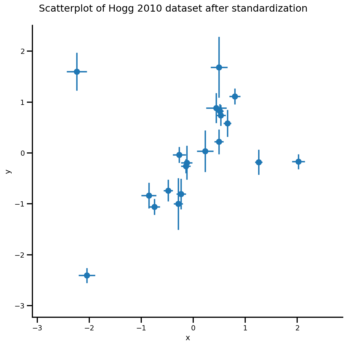
def plot_hoggs(dfhoggs):
## create xlims ylims for plotting
xlims = (dfhoggs['x'].min() - np.ptp(dfhoggs['x'])/5,
dfhoggs['x'].max() + np.ptp(dfhoggs['x'])/5)
ylims = (dfhoggs['y'].min() - np.ptp(dfhoggs['y'])/5,
dfhoggs['y'].max() + np.ptp(dfhoggs['y'])/5)
## scatterplot the standardized data
g = sns.FacetGrid(dfhoggs, size=8)
_ = g.map(plt.errorbar, 'x', 'y', 'sigma_y', 'sigma_x', marker="o", ls='')
_ = g.axes[0][0].set_ylim(ylims)
_ = g.axes[0][0].set_xlim(xlims)
plt.subplots_adjust(top=0.92)
_ = g.fig.suptitle('Scatterplot of Hogg 2010 dataset after standardization', fontsize=16)
return g, xlims, ylims
g = plot_hoggs(dfhoggs)
/usr/local/lib/python3.6/dist-packages/numpy/core/fromnumeric.py:2495: FutureWarning: Method .ptp is deprecated and will be removed in a future version. Use numpy.ptp instead.
  return ptp(axis=axis, out=out, **kwargs)
/usr/local/lib/python3.6/dist-packages/seaborn/axisgrid.py:230: UserWarning: The `size` paramter has been renamed to `height`; please update your code.
  warnings.warn(msg, UserWarning)
X_np = dfhoggs['x'].values
sigma_y_np = dfhoggs['sigma_y'].values
Y_np = dfhoggs['y'].values
Modello OLS convenzionale
Ora, impostiamo un modello lineare, un semplice problema di regressione intercetta + pendenza:
mdl_ols = tfd.JointDistributionSequential([
    # b0 ~ Normal(0, 1)
    tfd.Normal(loc=tf.cast(0, dtype), scale=1.),
    # b1 ~ Normal(0, 1)
    tfd.Normal(loc=tf.cast(0, dtype), scale=1.),
    # x ~ Normal(b0+b1*X, 1)
    lambda b1, b0: tfd.Normal(
      # Parameter transformation
      loc=b0 + b1*X_np,
      scale=sigma_y_np)
])
È quindi possibile controllare il grafico del modello per vedere la dipendenza. Si noti che x è riservato come il nome del l'ultimo nodo, e non è possibile che sia come il vostro argomento lambda nel modello JointDistributionSequential.
mdl_ols.resolve_graph()
(('b0', ()), ('b1', ()), ('x', ('b1', 'b0')))
Il campionamento dal modello è abbastanza semplice:
mdl_ols.sample()
[<tf.Tensor: shape=(), dtype=float64, numpy=-0.50225804634794>,
 <tf.Tensor: shape=(), dtype=float64, numpy=0.682740126293564>,
 <tf.Tensor: shape=(20,), dtype=float64, numpy=
 array([-0.33051382,  0.71443618, -1.91085683,  0.89371173, -0.45060957,
        -1.80448758, -0.21357082,  0.07891058, -0.20689721, -0.62690385,
        -0.55225748, -0.11446535, -0.66624497, -0.86913291, -0.93605552,
        -0.83965336, -0.70988597, -0.95813437,  0.15884761, -0.31113434])>]
...che fornisce un elenco di tf.Tensor. Puoi collegarlo immediatamente alla funzione log_prob per calcolare il log_prob del modello:
prior_predictive_samples = mdl_ols.sample()
mdl_ols.log_prob(prior_predictive_samples)
<tf.Tensor: shape=(20,), dtype=float64, numpy=
array([-4.97502846, -3.98544303, -4.37514505, -3.46933487, -3.80688125,
       -3.42907525, -4.03263074, -3.3646366 , -4.70370938, -4.36178501,
       -3.47823735, -3.94641662, -5.76906319, -4.0944128 , -4.39310708,
       -4.47713894, -4.46307881, -3.98802372, -3.83027747, -4.64777082])>
Hmmm, qualcosa non va qui: dovremmo ottenere un log_prob scalare! In effetti, possiamo ulteriormente controllare per vedere se qualcosa è fuori chiamando i .log_prob_parts , che dà la log_prob di ogni nodi del modello grafico:
mdl_ols.log_prob_parts(prior_predictive_samples)
[<tf.Tensor: shape=(), dtype=float64, numpy=-0.9699239562734849>,
 <tf.Tensor: shape=(), dtype=float64, numpy=-3.459364167569284>,
 <tf.Tensor: shape=(20,), dtype=float64, numpy=
 array([-0.54574034,  0.4438451 ,  0.05414307,  0.95995326,  0.62240687,
         1.00021288,  0.39665739,  1.06465152, -0.27442125,  0.06750311,
         0.95105078,  0.4828715 , -1.33977506,  0.33487533,  0.03618104,
        -0.04785082, -0.03379069,  0.4412644 ,  0.59901066, -0.2184827 ])>]
...si scopre che l'ultimo nodo non viene reduce_sum lungo l'iid dimensione/asse! Quando facciamo la somma, le prime due variabili vengono quindi trasmesse in modo errato.
Il trucco è quello di utilizzare tfd.Independent per reinterpretato forma batch (in modo che il resto dell'asse sarà ridotto correttamente):
mdl_ols_ = tfd.JointDistributionSequential([
    # b0
    tfd.Normal(loc=tf.cast(0, dtype), scale=1.),
    # b1
    tfd.Normal(loc=tf.cast(0, dtype), scale=1.),
    # likelihood
    #   Using Independent to ensure the log_prob is not incorrectly broadcasted
    lambda b1, b0: tfd.Independent(
        tfd.Normal(
            # Parameter transformation
            # b1 shape: (batch_shape), X shape (num_obs): we want result to have
            # shape (batch_shape, num_obs)
            loc=b0 + b1*X_np,
            scale=sigma_y_np),
        reinterpreted_batch_ndims=1
    ),
])
Ora, controlliamo l'ultimo nodo/distribuzione del modello, puoi vedere che la forma dell'evento è ora interpretata correttamente. Si noti che si potrebbe prendere un po 'di tentativi ed errori per ottenere i reinterpreted_batch_ndims destra, ma si può sempre stampare facilmente la distribuzione o il tensore di campionato al doppio controllo la forma!
print(mdl_ols_.sample_distributions()[0][-1])
print(mdl_ols.sample_distributions()[0][-1])
tfp.distributions.Independent("JointDistributionSequential_sample_distributions_IndependentJointDistributionSequential_sample_distributions_Normal", batch_shape=[], event_shape=[20], dtype=float64)
tfp.distributions.Normal("JointDistributionSequential_sample_distributions_Normal", batch_shape=[20], event_shape=[], dtype=float64)
prior_predictive_samples = mdl_ols_.sample()
mdl_ols_.log_prob(prior_predictive_samples)  # <== Getting a scalar correctly
<tf.Tensor: shape=(), dtype=float64, numpy=-2.543425661013286>
Altro JointDistribution* API
mdl_ols_named = tfd.JointDistributionNamed(dict(
    likelihood = lambda b0, b1: tfd.Independent(
        tfd.Normal(
            loc=b0 + b1*X_np,
            scale=sigma_y_np),
        reinterpreted_batch_ndims=1
    ),
    b0         = tfd.Normal(loc=tf.cast(0, dtype), scale=1.),
    b1         = tfd.Normal(loc=tf.cast(0, dtype), scale=1.),
))

mdl_ols_named.log_prob(mdl_ols_named.sample())
<tf.Tensor: shape=(), dtype=float64, numpy=-5.99620966071338>
mdl_ols_named.sample() # output is a dictionary
{'b0': <tf.Tensor: shape=(), dtype=float64, numpy=0.26364058399428225>,
 'b1': <tf.Tensor: shape=(), dtype=float64, numpy=-0.27209402374432207>,
 'likelihood': <tf.Tensor: shape=(20,), dtype=float64, numpy=
 array([ 0.6482155 , -0.39314108,  0.62744764, -0.24587987, -0.20544617,
         1.01465392, -0.04705611, -0.16618702,  0.36410134,  0.3943299 ,
         0.36455291, -0.27822219, -0.24423928,  0.24599518,  0.82731092,
        -0.21983033,  0.56753169,  0.32830481, -0.15713064,  0.23336351])>}
Root = tfd.JointDistributionCoroutine.Root  # Convenient alias.
def model():
  b1 = yield Root(tfd.Normal(loc=tf.cast(0, dtype), scale=1.))
  b0 = yield Root(tfd.Normal(loc=tf.cast(0, dtype), scale=1.))
  yhat = b0 + b1*X_np
  likelihood = yield tfd.Independent(
        tfd.Normal(loc=yhat, scale=sigma_y_np),
        reinterpreted_batch_ndims=1
    )

mdl_ols_coroutine = tfd.JointDistributionCoroutine(model)
mdl_ols_coroutine.log_prob(mdl_ols_coroutine.sample())
<tf.Tensor: shape=(), dtype=float64, numpy=-4.566678123520463>
mdl_ols_coroutine.sample() # output is a tuple
(<tf.Tensor: shape=(), dtype=float64, numpy=0.06811002171170354>,
 <tf.Tensor: shape=(), dtype=float64, numpy=-0.37477064754116807>,
 <tf.Tensor: shape=(20,), dtype=float64, numpy=
 array([-0.91615096, -0.20244718, -0.47840159, -0.26632479, -0.60441105,
        -0.48977789, -0.32422329, -0.44019322, -0.17072643, -0.20666025,
        -0.55932191, -0.40801868, -0.66893181, -0.24134135, -0.50403536,
        -0.51788596, -0.90071876, -0.47382338, -0.34821655, -0.38559724])>)
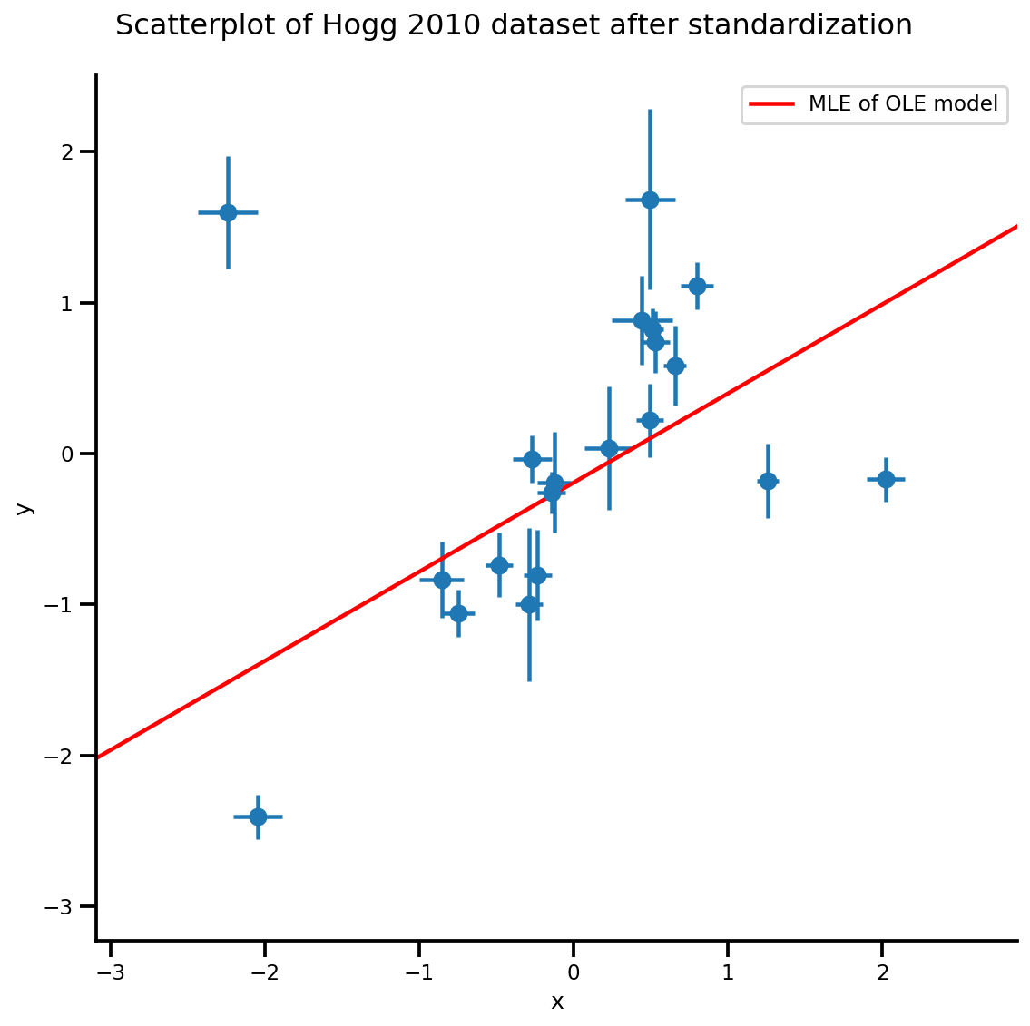
MLE
E ora possiamo fare inferenze! Puoi utilizzare l'ottimizzatore per trovare la stima della massima verosimiglianza.
Definire alcune funzioni di supporto
# bfgs and lbfgs currently requries a function that returns both the value and
# gradient re the input.
import functools

def _make_val_and_grad_fn(value_fn):
  @functools.wraps(value_fn)
  def val_and_grad(x):
    return tfp.math.value_and_gradient(value_fn, x)
  return val_and_grad

# Map a list of tensors (e.g., output from JDSeq.sample([...])) to a single tensor
# modify from tfd.Blockwise
from tensorflow_probability.python.internal import dtype_util
from tensorflow_probability.python.internal import prefer_static as ps
from tensorflow_probability.python.internal import tensorshape_util

class Mapper:
  """Basically, this is a bijector without log-jacobian correction."""
  def __init__(self, list_of_tensors, list_of_bijectors, event_shape):
    self.dtype = dtype_util.common_dtype(
        list_of_tensors, dtype_hint=tf.float32)
    self.list_of_tensors = list_of_tensors
    self.bijectors = list_of_bijectors
    self.event_shape = event_shape

  def flatten_and_concat(self, list_of_tensors):
    def _reshape_map_part(part, event_shape, bijector):
      part = tf.cast(bijector.inverse(part), self.dtype)
      static_rank = tf.get_static_value(ps.rank_from_shape(event_shape))
      if static_rank == 1:
        return part
      new_shape = ps.concat([
          ps.shape(part)[:ps.size(ps.shape(part)) - ps.size(event_shape)],
          [-1]
      ], axis=-1)
      return tf.reshape(part, ps.cast(new_shape, tf.int32))

    x = tf.nest.map_structure(_reshape_map_part,
                              list_of_tensors,
                              self.event_shape,
                              self.bijectors)
    return tf.concat(tf.nest.flatten(x), axis=-1)

  def split_and_reshape(self, x):
    assertions = []
    message = 'Input must have at least one dimension.'
    if tensorshape_util.rank(x.shape) is not None:
      if tensorshape_util.rank(x.shape) == 0:
        raise ValueError(message)
    else:
      assertions.append(assert_util.assert_rank_at_least(x, 1, message=message))
    with tf.control_dependencies(assertions):
      splits = [
          tf.cast(ps.maximum(1, ps.reduce_prod(s)), tf.int32)
          for s in tf.nest.flatten(self.event_shape)
      ]
      x = tf.nest.pack_sequence_as(
          self.event_shape, tf.split(x, splits, axis=-1))
      def _reshape_map_part(part, part_org, event_shape, bijector):
        part = tf.cast(bijector.forward(part), part_org.dtype)
        static_rank = tf.get_static_value(ps.rank_from_shape(event_shape))
        if static_rank == 1:
          return part
        new_shape = ps.concat([ps.shape(part)[:-1], event_shape], axis=-1)
        return tf.reshape(part, ps.cast(new_shape, tf.int32))

      x = tf.nest.map_structure(_reshape_map_part,
                                x,
                                self.list_of_tensors,
                                self.event_shape,
                                self.bijectors)
    return x
mapper = Mapper(mdl_ols_.sample()[:-1],
                [tfb.Identity(), tfb.Identity()],
                mdl_ols_.event_shape[:-1])

# mapper.split_and_reshape(mapper.flatten_and_concat(mdl_ols_.sample()[:-1]))
@_make_val_and_grad_fn
def neg_log_likelihood(x):
  # Generate a function closure so that we are computing the log_prob
  # conditioned on the observed data. Note also that tfp.optimizer.* takes a
  # single tensor as input.
  return -mdl_ols_.log_prob(mapper.split_and_reshape(x) + [Y_np])

lbfgs_results = tfp.optimizer.lbfgs_minimize(
    neg_log_likelihood,
    initial_position=tf.zeros(2, dtype=dtype),
    tolerance=1e-20,
    x_tolerance=1e-8
)
b0est, b1est = lbfgs_results.position.numpy()

g, xlims, ylims = plot_hoggs(dfhoggs);
xrange = np.linspace(xlims[0], xlims[1], 100)
g.axes[0][0].plot(xrange, b0est + b1est*xrange,
                  color='r', label='MLE of OLE model')
plt.legend();
/usr/local/lib/python3.6/dist-packages/numpy/core/fromnumeric.py:2495: FutureWarning: Method .ptp is deprecated and will be removed in a future version. Use numpy.ptp instead.
  return ptp(axis=axis, out=out, **kwargs)
/usr/local/lib/python3.6/dist-packages/seaborn/axisgrid.py:230: UserWarning: The `size` paramter has been renamed to `height`; please update your code.
  warnings.warn(msg, UserWarning)
Modello versione batch e MCMC
In bayesiana inferenza, di solito vogliamo lavorare con i campioni MCMC, come quando i campioni sono dalla parte posteriore, li può essere inserita in qualsiasi funzione delle aspettative di calcolo. Tuttavia, il MCMC API ci impongono di scrivere modelli che sono in batch cordiale, e siamo in grado di verificare che il nostro modello non è in realtà "batchable" chiamando il sample([...])
mdl_ols_.sample(5) # <== error as some computation could not be broadcasted.
In questo caso, è relativamente semplice poiché abbiamo solo una funzione lineare all'interno del nostro modello, espandere la forma dovrebbe fare il trucco:
mdl_ols_batch = tfd.JointDistributionSequential([
    # b0
    tfd.Normal(loc=tf.cast(0, dtype), scale=1.),
    # b1
    tfd.Normal(loc=tf.cast(0, dtype), scale=1.),
    # likelihood
    #   Using Independent to ensure the log_prob is not incorrectly broadcasted
    lambda b1, b0: tfd.Independent(
        tfd.Normal(
            # Parameter transformation
            loc=b0[..., tf.newaxis] + b1[..., tf.newaxis]*X_np[tf.newaxis, ...],
            scale=sigma_y_np[tf.newaxis, ...]),
        reinterpreted_batch_ndims=1
    ),
])

mdl_ols_batch.resolve_graph()
(('b0', ()), ('b1', ()), ('x', ('b1', 'b0')))
Possiamo nuovamente campionare e valutare log_prob_parts per eseguire alcuni controlli:
b0, b1, y = mdl_ols_batch.sample(4)
mdl_ols_batch.log_prob_parts([b0, b1, y])
[<tf.Tensor: shape=(4,), dtype=float64, numpy=array([-1.25230168, -1.45281432, -1.87110061, -1.07665206])>,
 <tf.Tensor: shape=(4,), dtype=float64, numpy=array([-1.07019936, -1.59562117, -2.53387765, -1.01557632])>,
 <tf.Tensor: shape=(4,), dtype=float64, numpy=array([ 0.45841406,  2.56829635, -4.84973951, -5.59423992])>]
Alcune note a margine:
- Vogliamo lavorare con la versione batch del modello perché è la più veloce per MCMC multi-catena. Nei casi che non si può riscrivere il modello come una versione in batch (per esempio, modelli ODE), è possibile associare la funzione log_prob utilizzando
tf.map_fnper ottenere lo stesso effetto. - Ora
mdl_ols_batch.sample()potrebbe non funzionare come abbiamo scaler prima, come non si può farescaler_tensor[:, None]. La soluzione è quella di ampliare scaler tensore di rango 1 avvolgendotfd.Sample(..., sample_shape=1). - È una buona pratica scrivere il modello come una funzione in modo da poter modificare le impostazioni come gli iperparametri molto più facilmente.
def gen_ols_batch_model(X, sigma, hyperprior_mean=0, hyperprior_scale=1):
  hyper_mean = tf.cast(hyperprior_mean, dtype)
  hyper_scale = tf.cast(hyperprior_scale, dtype)
  return tfd.JointDistributionSequential([
      # b0
      tfd.Sample(tfd.Normal(loc=hyper_mean, scale=hyper_scale), sample_shape=1),
      # b1
      tfd.Sample(tfd.Normal(loc=hyper_mean, scale=hyper_scale), sample_shape=1),
      # likelihood
      lambda b1, b0: tfd.Independent(
          tfd.Normal(
              # Parameter transformation
              loc=b0 + b1*X,
              scale=sigma),
          reinterpreted_batch_ndims=1
      ),
  ], validate_args=True)

mdl_ols_batch = gen_ols_batch_model(X_np[tf.newaxis, ...],
                                    sigma_y_np[tf.newaxis, ...])

_ = mdl_ols_batch.sample()
_ = mdl_ols_batch.sample(4)
_ = mdl_ols_batch.sample([3, 4])
# Small helper function to validate log_prob shape (avoid wrong broadcasting)
def validate_log_prob_part(model, batch_shape=1, observed=-1):
  samples = model.sample(batch_shape)
  logp_part = list(model.log_prob_parts(samples))

  # exclude observed node
  logp_part.pop(observed)
  for part in logp_part:
    tf.assert_equal(part.shape, logp_part[-1].shape)

validate_log_prob_part(mdl_ols_batch, 4)
Ulteriori controlli: confronto della funzione log_prob generata con la funzione log_prob TFP scritta a mano.
def ols_logp_batch(b0, b1, Y):
  b0_prior = tfd.Normal(loc=tf.cast(0, dtype), scale=1.) # b0
  b1_prior = tfd.Normal(loc=tf.cast(0, dtype), scale=1.) # b1
  likelihood = tfd.Normal(loc=b0 + b1*X_np[None, :],
                          scale=sigma_y_np) # likelihood
  return tf.reduce_sum(b0_prior.log_prob(b0), axis=-1) +\
         tf.reduce_sum(b1_prior.log_prob(b1), axis=-1) +\
         tf.reduce_sum(likelihood.log_prob(Y), axis=-1)

b0, b1, x = mdl_ols_batch.sample(4)
print(mdl_ols_batch.log_prob([b0, b1, Y_np]).numpy())
print(ols_logp_batch(b0, b1, Y_np).numpy())
[-227.37899384 -327.10043743 -570.44162789 -702.79808683]
[-227.37899384 -327.10043743 -570.44162789 -702.79808683]
MCMC con il campionatore senza inversione di marcia
Un comune run_chain funzione
@tf.function(autograph=False, experimental_compile=True)
def run_chain(init_state, step_size, target_log_prob_fn, unconstraining_bijectors,
              num_steps=500, burnin=50):

  def trace_fn(_, pkr):
    return (
        pkr.inner_results.inner_results.target_log_prob,
        pkr.inner_results.inner_results.leapfrogs_taken,
        pkr.inner_results.inner_results.has_divergence,
        pkr.inner_results.inner_results.energy,
        pkr.inner_results.inner_results.log_accept_ratio
           )

  kernel = tfp.mcmc.TransformedTransitionKernel(
    inner_kernel=tfp.mcmc.NoUTurnSampler(
      target_log_prob_fn,
      step_size=step_size),
    bijector=unconstraining_bijectors)

  hmc = tfp.mcmc.DualAveragingStepSizeAdaptation(
    inner_kernel=kernel,
    num_adaptation_steps=burnin,
    step_size_setter_fn=lambda pkr, new_step_size: pkr._replace(
        inner_results=pkr.inner_results._replace(step_size=new_step_size)),
    step_size_getter_fn=lambda pkr: pkr.inner_results.step_size,
    log_accept_prob_getter_fn=lambda pkr: pkr.inner_results.log_accept_ratio
  )

  # Sampling from the chain.
  chain_state, sampler_stat = tfp.mcmc.sample_chain(
      num_results=num_steps,
      num_burnin_steps=burnin,
      current_state=init_state,
      kernel=hmc,
      trace_fn=trace_fn)
  return chain_state, sampler_stat
nchain = 10
b0, b1, _ = mdl_ols_batch.sample(nchain)
init_state = [b0, b1]
step_size = [tf.cast(i, dtype=dtype) for i in [.1, .1]]
target_log_prob_fn = lambda *x: mdl_ols_batch.log_prob(x + (Y_np, ))

# bijector to map contrained parameters to real
unconstraining_bijectors = [
    tfb.Identity(),
    tfb.Identity(),
]

samples, sampler_stat = run_chain(
    init_state, step_size, target_log_prob_fn, unconstraining_bijectors)
# using the pymc3 naming convention
sample_stats_name = ['lp', 'tree_size', 'diverging', 'energy', 'mean_tree_accept']
sample_stats = {k:v.numpy().T for k, v in zip(sample_stats_name, sampler_stat)}
sample_stats['tree_size'] = np.diff(sample_stats['tree_size'], axis=1)
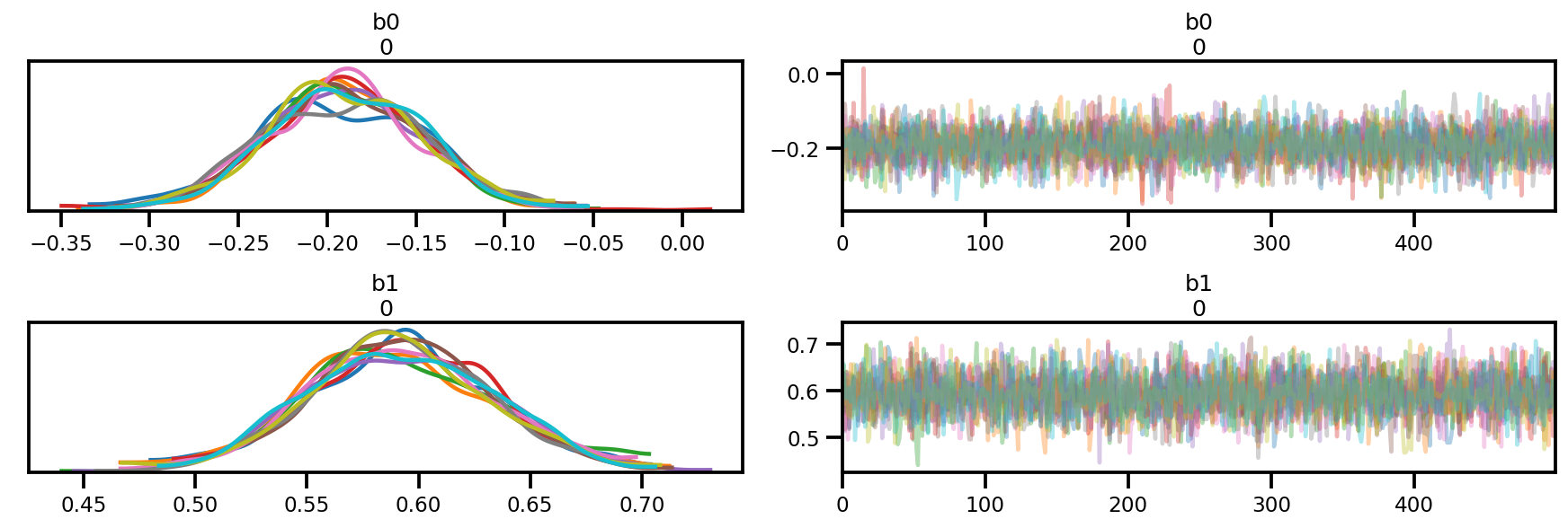
var_name = ['b0', 'b1']
posterior = {k:np.swapaxes(v.numpy(), 1, 0)
for k, v in zip(var_name, samples)}
az_trace = az.from_dict(posterior=posterior, sample_stats=sample_stats)
az.plot_trace(az_trace);
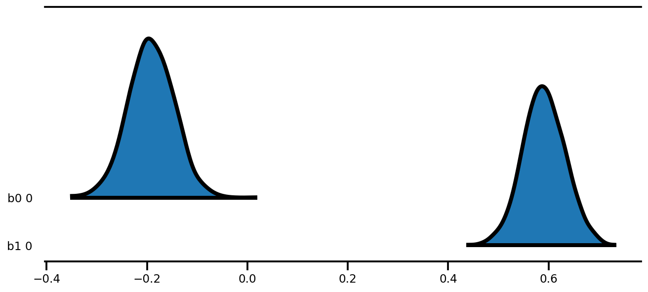
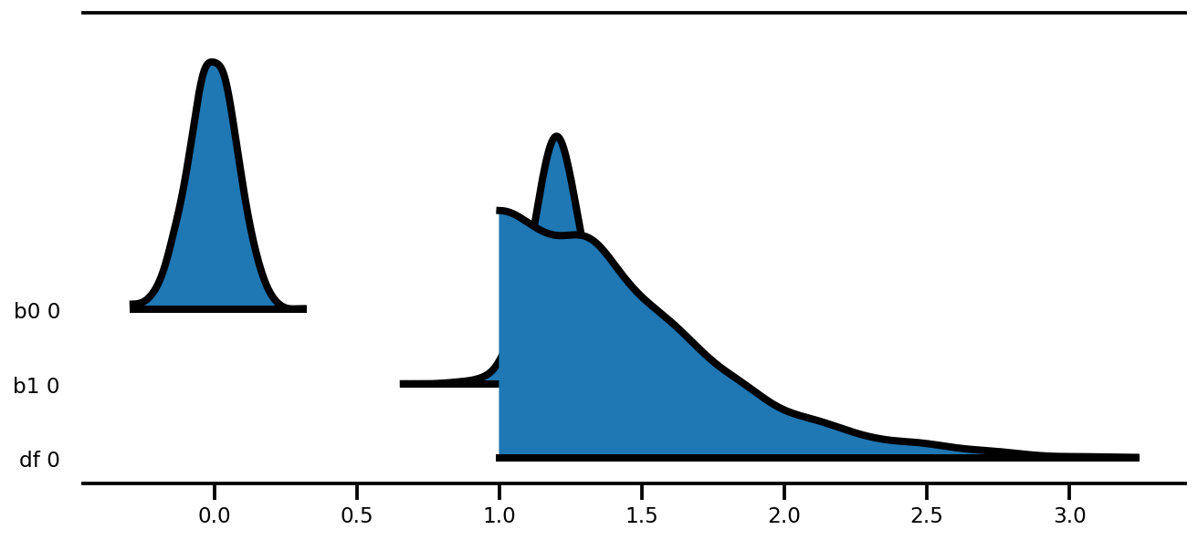
az.plot_forest(az_trace,
               kind='ridgeplot',
               linewidth=4,
               combined=True,
               ridgeplot_overlap=1.5,
               figsize=(9, 4));
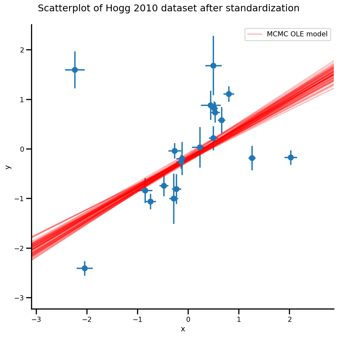
k = 5
b0est, b1est = az_trace.posterior['b0'][:, -k:].values, az_trace.posterior['b1'][:, -k:].values

g, xlims, ylims = plot_hoggs(dfhoggs);
xrange = np.linspace(xlims[0], xlims[1], 100)[None, :]
g.axes[0][0].plot(np.tile(xrange, (k, 1)).T,
                  (np.reshape(b0est, [-1, 1]) + np.reshape(b1est, [-1, 1])*xrange).T,
                  alpha=.25, color='r')
plt.legend([g.axes[0][0].lines[-1]], ['MCMC OLE model']);
/usr/local/lib/python3.6/dist-packages/numpy/core/fromnumeric.py:2495: FutureWarning: Method .ptp is deprecated and will be removed in a future version. Use numpy.ptp instead.
  return ptp(axis=axis, out=out, **kwargs)
/usr/local/lib/python3.6/dist-packages/seaborn/axisgrid.py:230: UserWarning: The `size` paramter has been renamed to `height`; please update your code.
  warnings.warn(msg, UserWarning)
/usr/local/lib/python3.6/dist-packages/ipykernel_launcher.py:8: MatplotlibDeprecationWarning: cycling among columns of inputs with non-matching shapes is deprecated.
Metodo Student-T
Nota che d'ora in poi lavoriamo sempre con la versione batch di un modello
def gen_studentt_model(X, sigma,
                       hyper_mean=0, hyper_scale=1, lower=1, upper=100):
  loc = tf.cast(hyper_mean, dtype)
  scale = tf.cast(hyper_scale, dtype)
  low = tf.cast(lower, dtype)
  high = tf.cast(upper, dtype)
  return tfd.JointDistributionSequential([
      # b0 ~ Normal(0, 1)
      tfd.Sample(tfd.Normal(loc, scale), sample_shape=1),
      # b1 ~ Normal(0, 1)
      tfd.Sample(tfd.Normal(loc, scale), sample_shape=1),
      # df ~ Uniform(a, b)
      tfd.Sample(tfd.Uniform(low, high), sample_shape=1),
      # likelihood ~ StudentT(df, f(b0, b1), sigma_y)
      #   Using Independent to ensure the log_prob is not incorrectly broadcasted.
      lambda df, b1, b0: tfd.Independent(
          tfd.StudentT(df=df, loc=b0 + b1*X, scale=sigma)),
  ], validate_args=True)

mdl_studentt = gen_studentt_model(X_np[tf.newaxis, ...],
                                  sigma_y_np[tf.newaxis, ...])
mdl_studentt.resolve_graph()
(('b0', ()), ('b1', ()), ('df', ()), ('x', ('df', 'b1', 'b0')))
validate_log_prob_part(mdl_studentt, 4)
Campione in avanti (campionamento predittivo precedente)
b0, b1, df, x = mdl_studentt.sample(1000)
x.shape
TensorShape([1000, 20])
MLE
# bijector to map contrained parameters to real
a, b = tf.constant(1., dtype), tf.constant(100., dtype),

# Interval transformation
tfp_interval = tfb.Inline(
    inverse_fn=(
        lambda x: tf.math.log(x - a) - tf.math.log(b - x)),
    forward_fn=(
        lambda y: (b - a) * tf.sigmoid(y) + a),
    forward_log_det_jacobian_fn=(
        lambda x: tf.math.log(b - a) - 2 * tf.nn.softplus(-x) - x),
    forward_min_event_ndims=0,
    name="interval")

unconstraining_bijectors = [
    tfb.Identity(),
    tfb.Identity(),
    tfp_interval,
]

mapper = Mapper(mdl_studentt.sample()[:-1],
                unconstraining_bijectors,
                mdl_studentt.event_shape[:-1])
@_make_val_and_grad_fn
def neg_log_likelihood(x):
  # Generate a function closure so that we are computing the log_prob
  # conditioned on the observed data. Note also that tfp.optimizer.* takes a
  # single tensor as input, so we need to do some slicing here:
  return -tf.squeeze(mdl_studentt.log_prob(
      mapper.split_and_reshape(x) + [Y_np]))

lbfgs_results = tfp.optimizer.lbfgs_minimize(
    neg_log_likelihood,
    initial_position=mapper.flatten_and_concat(mdl_studentt.sample()[:-1]),
    tolerance=1e-20,
    x_tolerance=1e-20
)
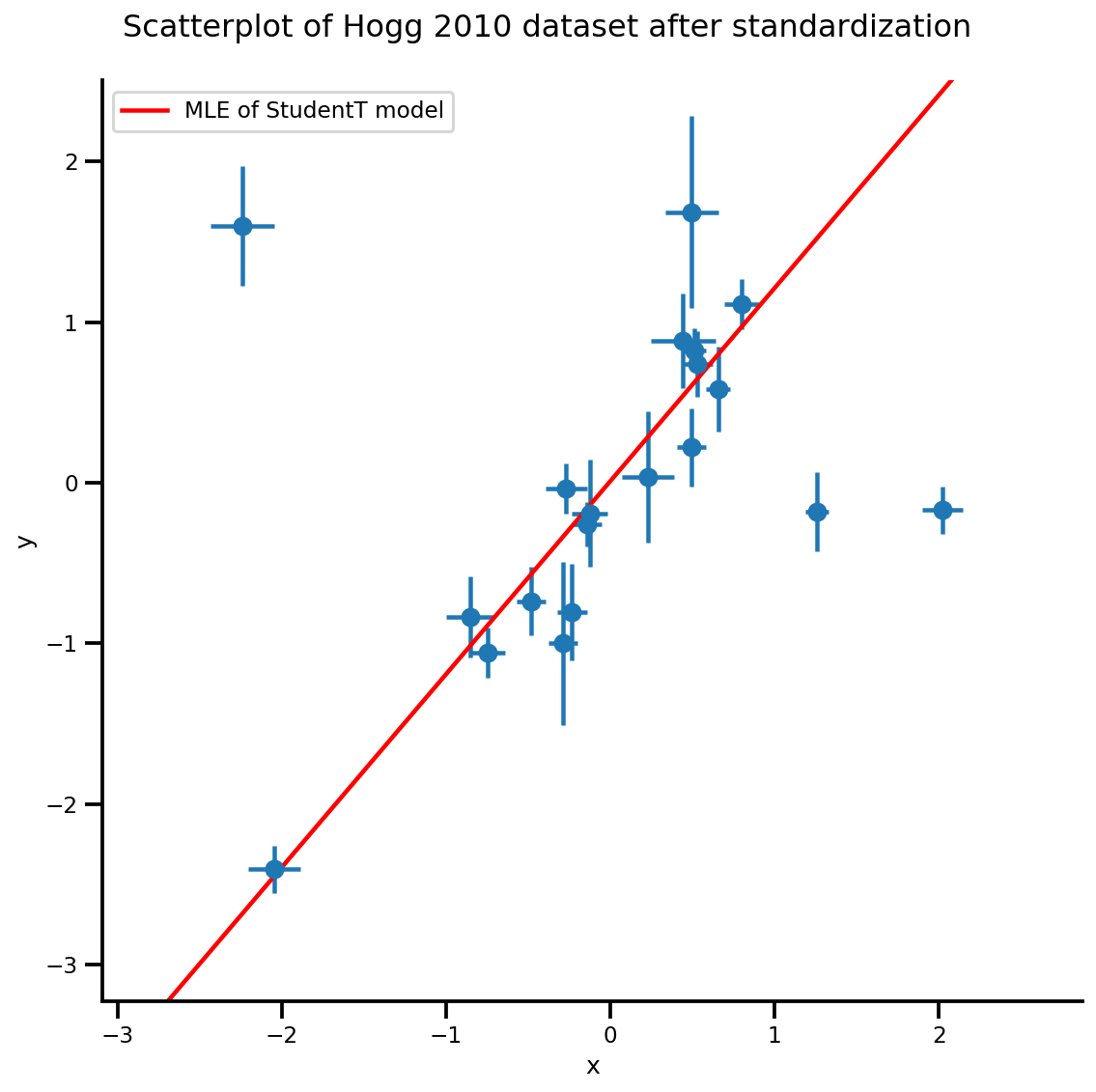
b0est, b1est, dfest = lbfgs_results.position.numpy()

g, xlims, ylims = plot_hoggs(dfhoggs);
xrange = np.linspace(xlims[0], xlims[1], 100)
g.axes[0][0].plot(xrange, b0est + b1est*xrange,
                  color='r', label='MLE of StudentT model')
plt.legend();
/usr/local/lib/python3.6/dist-packages/numpy/core/fromnumeric.py:2495: FutureWarning: Method .ptp is deprecated and will be removed in a future version. Use numpy.ptp instead.
  return ptp(axis=axis, out=out, **kwargs)
/usr/local/lib/python3.6/dist-packages/seaborn/axisgrid.py:230: UserWarning: The `size` paramter has been renamed to `height`; please update your code.
  warnings.warn(msg, UserWarning)
MCMC
nchain = 10
b0, b1, df, _ = mdl_studentt.sample(nchain)
init_state = [b0, b1, df]
step_size = [tf.cast(i, dtype=dtype) for i in [.1, .1, .05]]

target_log_prob_fn = lambda *x: mdl_studentt.log_prob(x + (Y_np, ))

samples, sampler_stat = run_chain(
    init_state, step_size, target_log_prob_fn, unconstraining_bijectors, burnin=100)
# using the pymc3 naming convention
sample_stats_name = ['lp', 'tree_size', 'diverging', 'energy', 'mean_tree_accept']
sample_stats = {k:v.numpy().T for k, v in zip(sample_stats_name, sampler_stat)}
sample_stats['tree_size'] = np.diff(sample_stats['tree_size'], axis=1)
var_name = ['b0', 'b1', 'df']
posterior = {k:np.swapaxes(v.numpy(), 1, 0)
for k, v in zip(var_name, samples)}
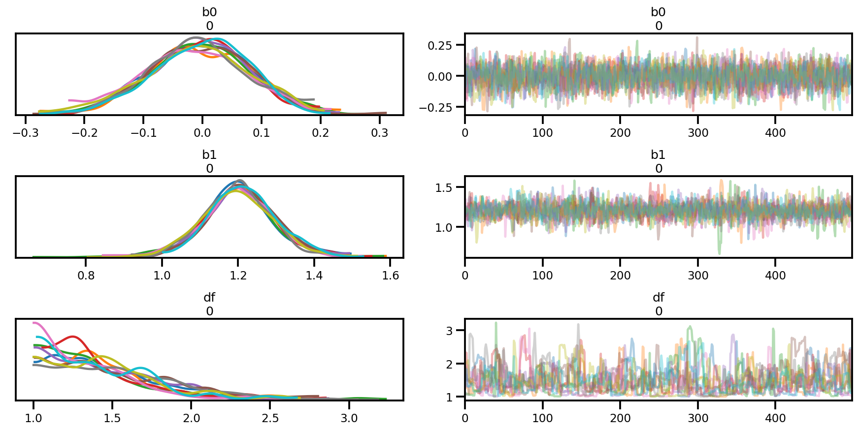
az_trace = az.from_dict(posterior=posterior, sample_stats=sample_stats)
az.summary(az_trace)
az.plot_trace(az_trace);
az.plot_forest(az_trace,
               kind='ridgeplot',
               linewidth=4,
               combined=True,
               ridgeplot_overlap=1.5,
               figsize=(9, 4));
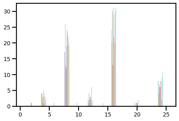
plt.hist(az_trace.sample_stats['tree_size'], np.linspace(.5, 25.5, 26), alpha=.5);
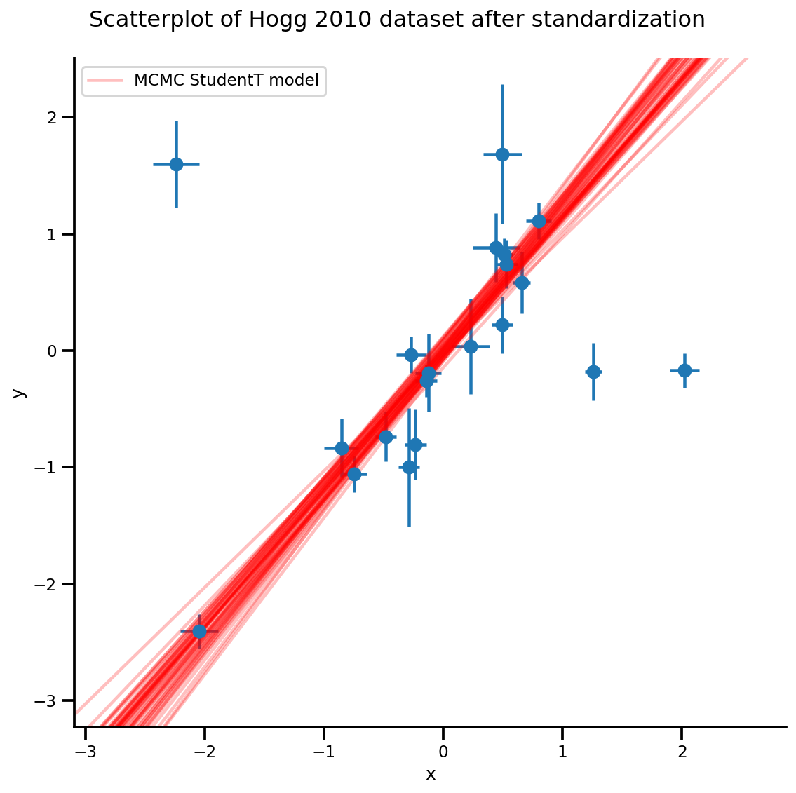
k = 5
b0est, b1est = az_trace.posterior['b0'][:, -k:].values, az_trace.posterior['b1'][:, -k:].values

g, xlims, ylims = plot_hoggs(dfhoggs);
xrange = np.linspace(xlims[0], xlims[1], 100)[None, :]
g.axes[0][0].plot(np.tile(xrange, (k, 1)).T,
                  (np.reshape(b0est, [-1, 1]) + np.reshape(b1est, [-1, 1])*xrange).T,
                  alpha=.25, color='r')
plt.legend([g.axes[0][0].lines[-1]], ['MCMC StudentT model']);
/usr/local/lib/python3.6/dist-packages/numpy/core/fromnumeric.py:2495: FutureWarning: Method .ptp is deprecated and will be removed in a future version. Use numpy.ptp instead.
  return ptp(axis=axis, out=out, **kwargs)
/usr/local/lib/python3.6/dist-packages/seaborn/axisgrid.py:230: UserWarning: The `size` paramter has been renamed to `height`; please update your code.
  warnings.warn(msg, UserWarning)
/usr/local/lib/python3.6/dist-packages/ipykernel_launcher.py:8: MatplotlibDeprecationWarning: cycling among columns of inputs with non-matching shapes is deprecated.
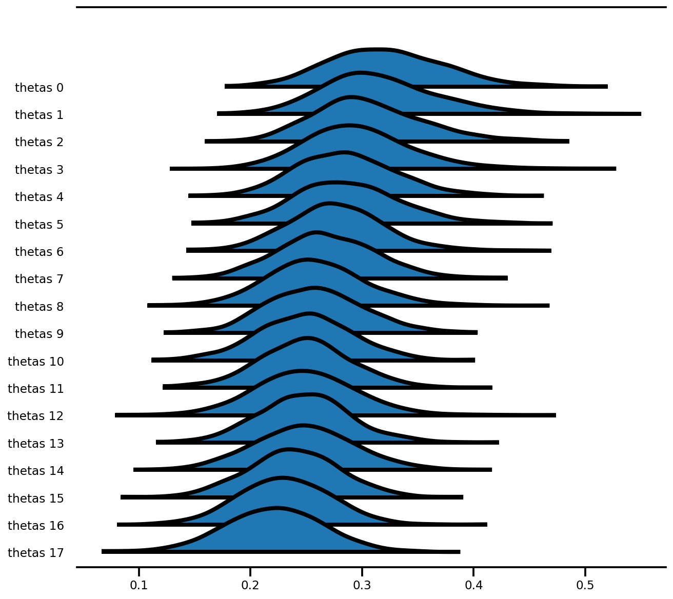
Raggruppamento parziale gerarchico
Da PyMC3 dati di baseball per 18 giocatori provenienti da Efron e Morris (1975)
data = pd.read_table('https://raw.githubusercontent.com/pymc-devs/pymc3/master/pymc3/examples/data/efron-morris-75-data.tsv',
                     sep="\t")
at_bats, hits = data[['At-Bats', 'Hits']].values.T
n = len(at_bats)
def gen_baseball_model(at_bats, rate=1.5, a=0, b=1):
  return tfd.JointDistributionSequential([
    # phi
    tfd.Uniform(low=tf.cast(a, dtype), high=tf.cast(b, dtype)),
    # kappa_log
    tfd.Exponential(rate=tf.cast(rate, dtype)),
    # thetas
    lambda kappa_log, phi: tfd.Sample(
        tfd.Beta(
            concentration1=tf.exp(kappa_log)*phi,
            concentration0=tf.exp(kappa_log)*(1.0-phi)),
        sample_shape=n
    ),
    # likelihood
    lambda thetas: tfd.Independent(
        tfd.Binomial(
            total_count=tf.cast(at_bats, dtype),
            probs=thetas
        )),
])

mdl_baseball = gen_baseball_model(at_bats)
mdl_baseball.resolve_graph()
(('phi', ()),
 ('kappa_log', ()),
 ('thetas', ('kappa_log', 'phi')),
 ('x', ('thetas',)))
Campione in avanti (campionamento predittivo precedente)
phi, kappa_log, thetas, y = mdl_baseball.sample(4)
# phi, kappa_log, thetas, y
Di nuovo, nota come se non usi Independent ti ritroverai con log_prob che ha batch_shape sbagliato.
# check logp
pprint(mdl_baseball.log_prob_parts([phi, kappa_log, thetas, hits]))
print(mdl_baseball.log_prob([phi, kappa_log, thetas, hits]))
[<tf.Tensor: shape=(4,), dtype=float64, numpy=array([0., 0., 0., 0.])>,
 <tf.Tensor: shape=(4,), dtype=float64, numpy=array([ 0.1721297 , -0.95946498, -0.72591188,  0.23993813])>,
 <tf.Tensor: shape=(4,), dtype=float64, numpy=array([59.35192283,  7.0650634 ,  0.83744911, 74.14370935])>,
 <tf.Tensor: shape=(4,), dtype=float64, numpy=array([-3279.75191016,  -931.10438484,  -512.59197688, -1131.08043597])>]
tf.Tensor([-3220.22785762  -924.99878641  -512.48043966 -1056.69678849], shape=(4,), dtype=float64)
MLE
Una caratteristica piuttosto sorprendente di tfp.optimizer è che, si può ottimizzato in parallelo per k lotto di punto di partenza e specificare lo stopping_condition kwarg: è possibile impostare a tfp.optimizer.converged_all per vedere se tutti trovano la stessa minimale, o tfp.optimizer.converged_any di trovare una soluzione locale veloce.
unconstraining_bijectors = [
    tfb.Sigmoid(),
    tfb.Exp(),
    tfb.Sigmoid(),
]

phi, kappa_log, thetas, y = mdl_baseball.sample(10)

mapper = Mapper([phi, kappa_log, thetas],
                unconstraining_bijectors,
                mdl_baseball.event_shape[:-1])
@_make_val_and_grad_fn
def neg_log_likelihood(x):
  return -mdl_baseball.log_prob(mapper.split_and_reshape(x) + [hits])

start = mapper.flatten_and_concat([phi, kappa_log, thetas])

lbfgs_results = tfp.optimizer.lbfgs_minimize(
    neg_log_likelihood,
    num_correction_pairs=10,
    initial_position=start,
    # lbfgs actually can work in batch as well
    stopping_condition=tfp.optimizer.converged_any,
    tolerance=1e-50,
    x_tolerance=1e-50,
    parallel_iterations=10,
    max_iterations=200
)
lbfgs_results.converged.numpy(), lbfgs_results.failed.numpy()
(array([False, False, False, False, False, False, False, False, False,
        False]),
 array([ True,  True,  True,  True,  True,  True,  True,  True,  True,
         True]))
result = lbfgs_results.position[lbfgs_results.converged & ~lbfgs_results.failed]
result
<tf.Tensor: shape=(0, 20), dtype=float64, numpy=array([], shape=(0, 20), dtype=float64)>
LBFGS non converge.
if result.shape[0] > 0:
  phi_est, kappa_est, theta_est = mapper.split_and_reshape(result)
  phi_est, kappa_est, theta_est
MCMC
target_log_prob_fn = lambda *x: mdl_baseball.log_prob(x + (hits, ))

nchain = 4
phi, kappa_log, thetas, _ = mdl_baseball.sample(nchain)
init_state = [phi, kappa_log, thetas]
step_size=[tf.cast(i, dtype=dtype) for i in [.1, .1, .1]]

samples, sampler_stat = run_chain(
    init_state, step_size, target_log_prob_fn, unconstraining_bijectors,
    burnin=200)
# using the pymc3 naming convention
sample_stats_name = ['lp', 'tree_size', 'diverging', 'energy', 'mean_tree_accept']
sample_stats = {k:v.numpy().T for k, v in zip(sample_stats_name, sampler_stat)}
sample_stats['tree_size'] = np.diff(sample_stats['tree_size'], axis=1)

var_name = ['phi', 'kappa_log', 'thetas']
posterior = {k:np.swapaxes(v.numpy(), 1, 0)
             for k, v in zip(var_name, samples)}

az_trace = az.from_dict(posterior=posterior, sample_stats=sample_stats)
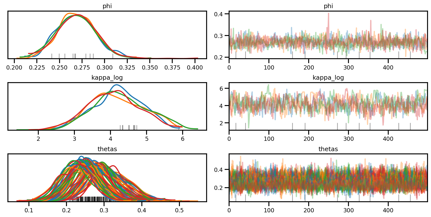
az.plot_trace(az_trace, compact=True);
az.plot_forest(az_trace,
               var_names=['thetas'],
               kind='ridgeplot',
               linewidth=4,
               combined=True,
               ridgeplot_overlap=1.5,
               figsize=(9, 8));
Modello ad effetto misto (Radon)
L'ultimo modello della doc PyMC3: A Primer su metodi bayesiani per Multilevel Modeling
Alcuni cambiamenti in precedenti (scala ridotta, ecc.)
Carica dati grezzi e pulisci
srrs2 = pd.read_csv('https://raw.githubusercontent.com/pymc-devs/pymc3/master/pymc3/examples/data/srrs2.dat')

srrs2.columns = srrs2.columns.map(str.strip)
srrs_mn = srrs2[srrs2.state=='MN'].copy()
srrs_mn['fips'] = srrs_mn.stfips*1000 + srrs_mn.cntyfips

cty = pd.read_csv('https://raw.githubusercontent.com/pymc-devs/pymc3/master/pymc3/examples/data/cty.dat')
cty_mn = cty[cty.st=='MN'].copy()
cty_mn[ 'fips'] = 1000*cty_mn.stfips + cty_mn.ctfips

srrs_mn = srrs_mn.merge(cty_mn[['fips', 'Uppm']], on='fips')
srrs_mn = srrs_mn.drop_duplicates(subset='idnum')
u = np.log(srrs_mn.Uppm)

n = len(srrs_mn)

srrs_mn.county = srrs_mn.county.map(str.strip)
mn_counties = srrs_mn.county.unique()
counties = len(mn_counties)
county_lookup = dict(zip(mn_counties, range(len(mn_counties))))

county = srrs_mn['county_code'] = srrs_mn.county.replace(county_lookup).values
radon = srrs_mn.activity
srrs_mn['log_radon'] = log_radon = np.log(radon + 0.1).values
floor_measure = srrs_mn.floor.values.astype('float')

# Create new variable for mean of floor across counties
xbar = srrs_mn.groupby('county')['floor'].mean().rename(county_lookup).values
Per i modelli con trasformazione complessa, implementarlo in uno stile funzionale renderebbe la scrittura e il test molto più semplici. Inoltre, rende molto più semplice generare a livello di programmazione la funzione log_prob che ha condizionato (mini-batch) i dati immessi:
def affine(u_val, x_county, county, floor, gamma, eps, b):
  """Linear equation of the coefficients and the covariates, with broadcasting."""
  return (tf.transpose((gamma[..., 0]
                      + gamma[..., 1]*u_val[:, None]
                      + gamma[..., 2]*x_county[:, None]))
          + tf.gather(eps, county, axis=-1)
          + b*floor)


def gen_radon_model(u_val, x_county, county, floor,
                    mu0=tf.zeros([], dtype, name='mu0')):
  """Creates a joint distribution representing our generative process."""
  return tfd.JointDistributionSequential([
      # sigma_a
      tfd.HalfCauchy(loc=mu0, scale=5.),
      # eps
      lambda sigma_a: tfd.Sample(
          tfd.Normal(loc=mu0, scale=sigma_a), sample_shape=counties),
      # gamma
      tfd.Sample(tfd.Normal(loc=mu0, scale=100.), sample_shape=3),
      # b
      tfd.Sample(tfd.Normal(loc=mu0, scale=100.), sample_shape=1),
      # sigma_y
      tfd.Sample(tfd.HalfCauchy(loc=mu0, scale=5.), sample_shape=1),
      # likelihood
      lambda sigma_y, b, gamma, eps: tfd.Independent(
          tfd.Normal(
              loc=affine(u_val, x_county, county, floor, gamma, eps, b),
              scale=sigma_y
          ),
          reinterpreted_batch_ndims=1
      ),
  ])

contextual_effect2 = gen_radon_model(
    u.values,  xbar[county], county, floor_measure)

@tf.function(autograph=False)
def unnormalized_posterior_log_prob(sigma_a, gamma, eps, b, sigma_y):
  """Computes `joint_log_prob` pinned at `log_radon`."""
  return contextual_effect2.log_prob(
      [sigma_a, gamma, eps, b, sigma_y, log_radon])

assert [4] == unnormalized_posterior_log_prob(
    *contextual_effect2.sample(4)[:-1]).shape
samples = contextual_effect2.sample(4)
pprint([s.shape for s in samples])
[TensorShape([4]),
 TensorShape([4, 85]),
 TensorShape([4, 3]),
 TensorShape([4, 1]),
 TensorShape([4, 1]),
 TensorShape([4, 919])]
contextual_effect2.log_prob_parts(list(samples)[:-1] + [log_radon])
[<tf.Tensor: shape=(4,), dtype=float64, numpy=array([-3.95681828, -2.45693443, -2.53310078, -4.7717536 ])>,
 <tf.Tensor: shape=(4,), dtype=float64, numpy=array([-340.65975204, -217.11139018, -246.50498667, -369.79687704])>,
 <tf.Tensor: shape=(4,), dtype=float64, numpy=array([-20.49822449, -20.38052557, -18.63843525, -17.83096972])>,
 <tf.Tensor: shape=(4,), dtype=float64, numpy=array([-5.94765605, -5.91460848, -6.66169402, -5.53894593])>,
 <tf.Tensor: shape=(4,), dtype=float64, numpy=array([-2.10293999, -4.34186631, -2.10744955, -3.016717  ])>,
 <tf.Tensor: shape=(4,), dtype=float64, numpy=
 array([-29022322.1413861 ,   -114422.36893361,  -8708500.81752865,
           -35061.92497235])>]
Inferenza variazionale
Una caratteristica molto potente di JointDistribution* è che si può generare un'approssimazione facilmente per VI. Ad esempio, per eseguire ADVI a campo medio, è sufficiente ispezionare il grafico e sostituire tutta la distribuzione non osservata con una distribuzione normale.
Meanfield ADVI
È anche possibile utilizzare la funzione experimential in tensorflow_probability / python / sperimentale / vi costruire approssimazione variazionale, che sono essenzialmente la stessa logica usata sotto (cioè, usando JointDistribution a costruire approssimazione), ma con l'uscita approssimazione nello spazio originale anziché la spazio illimitato.
from tensorflow_probability.python.mcmc.transformed_kernel import (
    make_transform_fn, make_transformed_log_prob)
# Wrap logp so that all parameters are in the Real domain
# copied and edited from tensorflow_probability/python/mcmc/transformed_kernel.py
unconstraining_bijectors = [
    tfb.Exp(),
    tfb.Identity(),
    tfb.Identity(),
    tfb.Identity(),
    tfb.Exp()
]

unnormalized_log_prob = lambda *x: contextual_effect2.log_prob(x + (log_radon,))

contextual_effect_posterior = make_transformed_log_prob(
    unnormalized_log_prob,
    unconstraining_bijectors,
    direction='forward',
    # TODO(b/72831017): Disable caching until gradient linkage
    # generally works.
    enable_bijector_caching=False)
# debug
if True:
  # Check the two versions of log_prob - they should be different given the Jacobian
  rv_samples = contextual_effect2.sample(4)

  _inverse_transform = make_transform_fn(unconstraining_bijectors, 'inverse')
  _forward_transform = make_transform_fn(unconstraining_bijectors, 'forward')

  pprint([
      unnormalized_log_prob(*rv_samples[:-1]),
      contextual_effect_posterior(*_inverse_transform(rv_samples[:-1])),
      unnormalized_log_prob(
          *_forward_transform(
              tf.zeros_like(a, dtype=dtype) for a in rv_samples[:-1])
      ),
      contextual_effect_posterior(
          *[tf.zeros_like(a, dtype=dtype) for a in rv_samples[:-1]]
      ),
  ])
[<tf.Tensor: shape=(4,), dtype=float64, numpy=array([-1.73354969e+04, -5.51622488e+04, -2.77754609e+08, -1.09065161e+07])>,
 <tf.Tensor: shape=(4,), dtype=float64, numpy=array([-1.73331358e+04, -5.51582029e+04, -2.77754602e+08, -1.09065134e+07])>,
 <tf.Tensor: shape=(4,), dtype=float64, numpy=array([-1992.10420767, -1992.10420767, -1992.10420767, -1992.10420767])>,
 <tf.Tensor: shape=(4,), dtype=float64, numpy=array([-1992.10420767, -1992.10420767, -1992.10420767, -1992.10420767])>]
# Build meanfield ADVI for a jointdistribution
# Inspect the input jointdistribution and replace the list of distribution with
# a list of Normal distribution, each with the same shape.
def build_meanfield_advi(jd_list, observed_node=-1):
  """
  The inputted jointdistribution needs to be a batch version
  """
  # Sample to get a list of Tensors
  list_of_values = jd_list.sample(1)  # <== sample([]) might not work

  # Remove the observed node
  list_of_values.pop(observed_node)

  # Iterate the list of Tensor to a build a list of Normal distribution (i.e.,
  # the Variational posterior)
  distlist = []
  for i, value in enumerate(list_of_values):
    dtype = value.dtype
    rv_shape = value[0].shape
    loc = tf.Variable(
        tf.random.normal(rv_shape, dtype=dtype),
        name='meanfield_%s_mu' % i,
        dtype=dtype)
    scale = tfp.util.TransformedVariable(
        tf.fill(rv_shape, value=tf.constant(0.02, dtype)),
        tfb.Softplus(),
        name='meanfield_%s_scale' % i,
    )

    approx_node = tfd.Normal(loc=loc, scale=scale)
    if loc.shape == ():
      distlist.append(approx_node)
    else:
      distlist.append(
          # TODO: make the reinterpreted_batch_ndims more flexible (for
          # minibatch etc)
          tfd.Independent(approx_node, reinterpreted_batch_ndims=1)
      )

  # pass list to JointDistribution to initiate the meanfield advi
  meanfield_advi = tfd.JointDistributionSequential(distlist)
  return meanfield_advi
advi = build_meanfield_advi(contextual_effect2, observed_node=-1)

# Check the logp and logq
advi_samples = advi.sample(4)
pprint([
  advi.log_prob(advi_samples),
  contextual_effect_posterior(*advi_samples)
  ])
[<tf.Tensor: shape=(4,), dtype=float64, numpy=array([231.26836839, 229.40755095, 227.10287879, 224.05914594])>,
 <tf.Tensor: shape=(4,), dtype=float64, numpy=array([-10615.93542431, -11743.21420129, -10376.26732337, -11338.00600103])>]
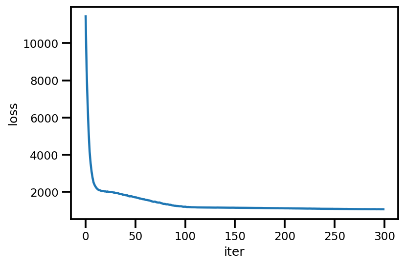
opt = tf.optimizers.Adam(learning_rate=.1)
@tf.function(experimental_compile=True)
def run_approximation():
loss_ = tfp.vi.fit_surrogate_posterior(
contextual_effect_posterior,
surrogate_posterior=advi,
optimizer=opt,
sample_size=10,
num_steps=300)
return loss_
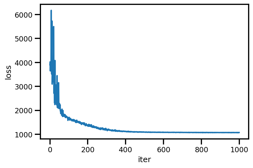
loss_ = run_approximation()
plt.plot(loss_);
plt.xlabel('iter');
plt.ylabel('loss');
graph_info = contextual_effect2.resolve_graph()
approx_param = dict()
free_param = advi.trainable_variables
for i, (rvname, param) in enumerate(graph_info[:-1]):
  approx_param[rvname] = {"mu": free_param[i*2].numpy(),
                          "sd": free_param[i*2+1].numpy()}
approx_param.keys()
dict_keys(['sigma_a', 'eps', 'gamma', 'b', 'sigma_y'])
approx_param['gamma']
{'mu': array([1.28145814, 0.70365287, 1.02689857]),
 'sd': array([-3.6604972 , -2.68153218, -2.04176524])}
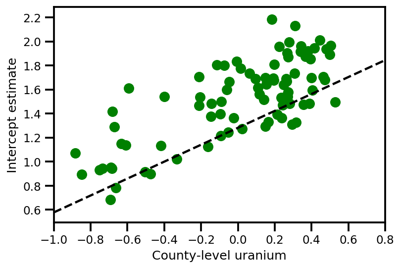
a_means = (approx_param['gamma']['mu'][0]
         + approx_param['gamma']['mu'][1]*u.values
         + approx_param['gamma']['mu'][2]*xbar[county]
         + approx_param['eps']['mu'][county])
_, index = np.unique(county, return_index=True)
plt.scatter(u.values[index], a_means[index], color='g')

xvals = np.linspace(-1, 0.8)
plt.plot(xvals,
         approx_param['gamma']['mu'][0]+approx_param['gamma']['mu'][1]*xvals,
         'k--')
plt.xlim(-1, 0.8)

plt.xlabel('County-level uranium');
plt.ylabel('Intercept estimate');
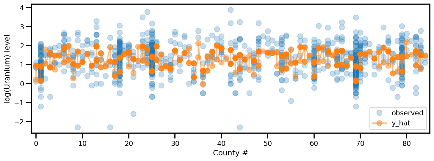
y_est = (approx_param['gamma']['mu'][0]
        + approx_param['gamma']['mu'][1]*u.values
        + approx_param['gamma']['mu'][2]*xbar[county]
        + approx_param['eps']['mu'][county]
        + approx_param['b']['mu']*floor_measure)

_, ax = plt.subplots(1, 1, figsize=(12, 4))
ax.plot(county, log_radon, 'o', alpha=.25, label='observed')
ax.plot(county, y_est, '-o', lw=2, alpha=.5, label='y_hat')
ax.set_xlim(-1, county.max()+1)
plt.legend(loc='lower right')
ax.set_xlabel('County #')
ax.set_ylabel('log(Uranium) level');
FullRank ADVI
Per ADVI di rango completo, vogliamo approssimare il posteriore con una gaussiana multivariata.
USE_FULLRANK = True
*prior_tensors, _ = contextual_effect2.sample()

mapper = Mapper(prior_tensors,
                [tfb.Identity() for _ in prior_tensors],
                contextual_effect2.event_shape[:-1])
rv_shape = ps.shape(mapper.flatten_and_concat(mapper.list_of_tensors))
init_val = tf.random.normal(rv_shape, dtype=dtype)
loc = tf.Variable(init_val, name='loc', dtype=dtype)

if USE_FULLRANK:
  # cov_param = tfp.util.TransformedVariable(
  #     10. * tf.eye(rv_shape[0], dtype=dtype),
  #     tfb.FillScaleTriL(),
  #     name='cov_param'
  #     )
  FillScaleTriL = tfb.FillScaleTriL(
        diag_bijector=tfb.Chain([
          tfb.Shift(tf.cast(.01, dtype)),
          tfb.Softplus(),
          tfb.Shift(tf.cast(np.log(np.expm1(1.)), dtype))]),
        diag_shift=None)
  cov_param = tfp.util.TransformedVariable(
      .02 * tf.eye(rv_shape[0], dtype=dtype),
      FillScaleTriL,
      name='cov_param')
  advi_approx = tfd.MultivariateNormalTriL(
      loc=loc, scale_tril=cov_param)
else:
  # An alternative way to build meanfield ADVI.
  cov_param = tfp.util.TransformedVariable(
      .02 * tf.ones(rv_shape, dtype=dtype),
      tfb.Softplus(),
      name='cov_param'
      )
  advi_approx = tfd.MultivariateNormalDiag(
      loc=loc, scale_diag=cov_param)

contextual_effect_posterior2 = lambda x: contextual_effect_posterior(
    *mapper.split_and_reshape(x)
)

# Check the logp and logq
advi_samples = advi_approx.sample(7)
pprint([
  advi_approx.log_prob(advi_samples),
  contextual_effect_posterior2(advi_samples)
  ])
[<tf.Tensor: shape=(7,), dtype=float64, numpy=
array([238.81841799, 217.71022639, 234.57207103, 230.0643819 ,
       243.73140943, 226.80149702, 232.85184209])>,
 <tf.Tensor: shape=(7,), dtype=float64, numpy=
array([-3638.93663169, -3664.25879314, -3577.69371677, -3696.25705312,
       -3689.12130489, -3777.53698383, -3659.4982734 ])>]
learning_rate = tf.optimizers.schedules.ExponentialDecay(
    initial_learning_rate=1e-2,
    decay_steps=10,
    decay_rate=0.99,
    staircase=True)

opt = tf.optimizers.Adam(learning_rate=learning_rate)

@tf.function(experimental_compile=True)
def run_approximation():
  loss_ = tfp.vi.fit_surrogate_posterior(
        contextual_effect_posterior2,
        surrogate_posterior=advi_approx,
        optimizer=opt,
        sample_size=10,
        num_steps=1000)
  return loss_

loss_ = run_approximation()
plt.plot(loss_);
plt.xlabel('iter');
plt.ylabel('loss');
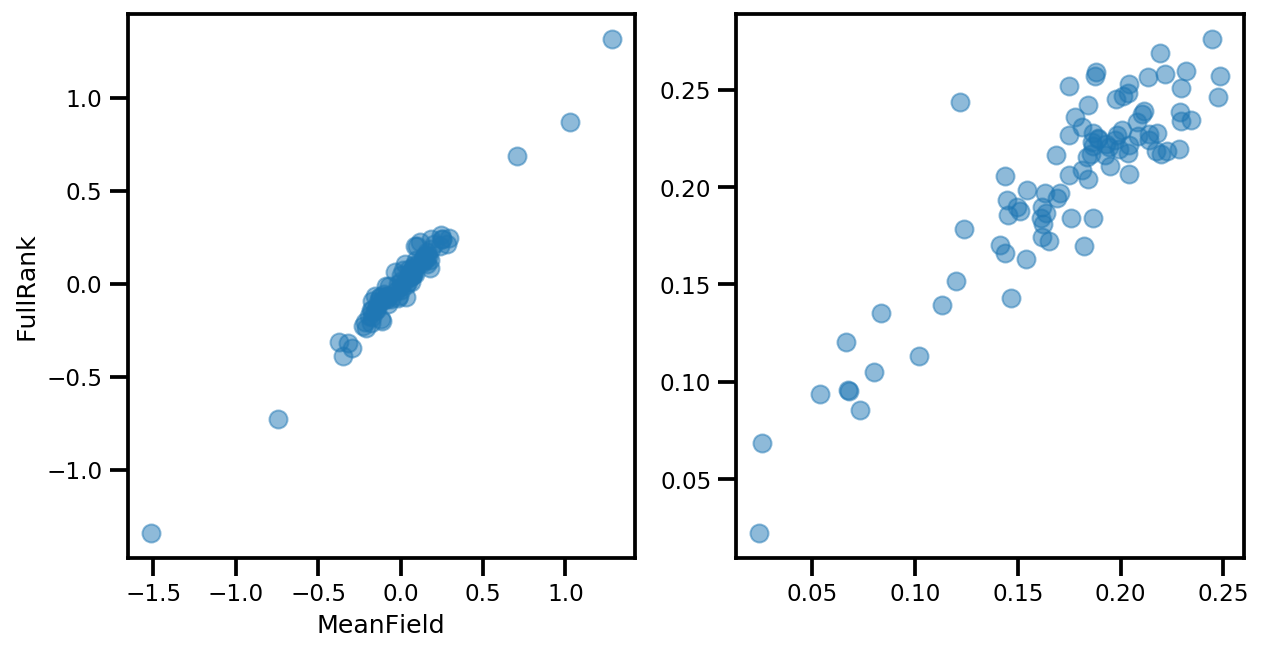
# debug
if True:
  _, ax = plt.subplots(1, 2, figsize=(10, 5))
  ax[0].plot(mapper.flatten_and_concat(advi.mean()), advi_approx.mean(), 'o', alpha=.5)
  ax[1].plot(mapper.flatten_and_concat(advi.stddev()), advi_approx.stddev(), 'o', alpha=.5)
  ax[0].set_xlabel('MeanField')
  ax[0].set_ylabel('FullRank')
graph_info = contextual_effect2.resolve_graph()
approx_param = dict()

free_param_mean = mapper.split_and_reshape(advi_approx.mean())
free_param_std = mapper.split_and_reshape(advi_approx.stddev())
for i, (rvname, param) in enumerate(graph_info[:-1]):
  approx_param[rvname] = {"mu": free_param_mean[i].numpy(),
                          "cov_info": free_param_std[i].numpy()}
a_means = (approx_param['gamma']['mu'][0]
         + approx_param['gamma']['mu'][1]*u.values
         + approx_param['gamma']['mu'][2]*xbar[county]
         + approx_param['eps']['mu'][county])
_, index = np.unique(county, return_index=True)
plt.scatter(u.values[index], a_means[index], color='g')

xvals = np.linspace(-1, 0.8)
plt.plot(xvals,
         approx_param['gamma']['mu'][0]+approx_param['gamma']['mu'][1]*xvals,
         'k--')
plt.xlim(-1, 0.8)

plt.xlabel('County-level uranium');
plt.ylabel('Intercept estimate');

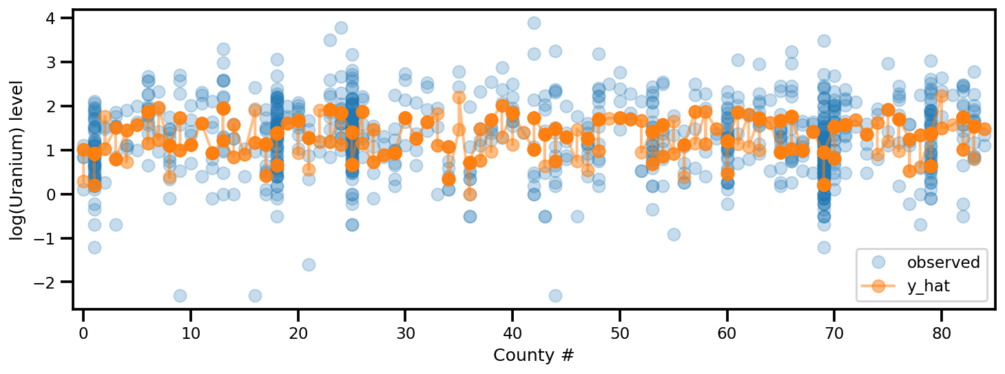
y_est = (approx_param['gamma']['mu'][0]
         + approx_param['gamma']['mu'][1]*u.values
         + approx_param['gamma']['mu'][2]*xbar[county]
         + approx_param['eps']['mu'][county]
         + approx_param['b']['mu']*floor_measure)

_, ax = plt.subplots(1, 1, figsize=(12, 4))
ax.plot(county, log_radon, 'o', alpha=.25, label='observed')
ax.plot(county, y_est, '-o', lw=2, alpha=.5, label='y_hat')
ax.set_xlim(-1, county.max()+1)
plt.legend(loc='lower right')
ax.set_xlabel('County #')
ax.set_ylabel('log(Uranium) level');
Modello di miscela beta-Bernoulli
Un modello misto in cui più revisori etichettano alcuni elementi, con etichette latenti (vere) sconosciute.
dtype = tf.float32
n = 50000    # number of examples reviewed
p_bad_ = 0.1 # fraction of bad events
m = 5        # number of reviewers for each example
rcl_ = .35 + np.random.rand(m)/10
prc_ = .65 + np.random.rand(m)/10

# PARAMETER TRANSFORMATION
tpr = rcl_
fpr = p_bad_*tpr*(1./prc_-1.)/(1.-p_bad_)
tnr = 1 - fpr

# broadcast to m reviewer.
batch_prob = np.asarray([tpr, fpr]).T
mixture = tfd.Mixture(
    tfd.Categorical(
        probs=[p_bad_, 1-p_bad_]),
    [
        tfd.Independent(tfd.Bernoulli(probs=tpr), 1),
        tfd.Independent(tfd.Bernoulli(probs=fpr), 1),
    ])
# Generate reviewer response
X_tf = mixture.sample([n])

# run once to always use the same array as input
# so we can compare the estimation from different
# inference method.
X_np = X_tf.numpy()
# batched Mixture model
mdl_mixture = tfd.JointDistributionSequential([
    tfd.Sample(tfd.Beta(5., 2.), m),
    tfd.Sample(tfd.Beta(2., 2.), m),
    tfd.Sample(tfd.Beta(1., 10), 1),
    lambda p_bad, rcl, prc: tfd.Sample(
        tfd.Mixture(
            tfd.Categorical(
                probs=tf.concat([p_bad, 1.-p_bad], -1)),
            [
              tfd.Independent(tfd.Bernoulli(
                  probs=rcl), 1),
              tfd.Independent(tfd.Bernoulli(
                  probs=p_bad*rcl*(1./prc-1.)/(1.-p_bad)), 1)
             ]
      ), (n, )),
    ])

mdl_mixture.resolve_graph()
(('prc', ()), ('rcl', ()), ('p_bad', ()), ('x', ('p_bad', 'rcl', 'prc')))
prc, rcl, p_bad, x = mdl_mixture.sample(4)
x.shape
TensorShape([4, 50000, 5])
mdl_mixture.log_prob_parts([prc, rcl, p_bad, X_np[np.newaxis, ...]])
[<tf.Tensor: shape=(4,), dtype=float32, numpy=array([1.4828572, 2.957961 , 2.9355168, 2.6116824], dtype=float32)>,
 <tf.Tensor: shape=(4,), dtype=float32, numpy=array([-0.14646745,  1.3308513 ,  1.1205603 ,  0.5441705 ], dtype=float32)>,
 <tf.Tensor: shape=(4,), dtype=float32, numpy=array([1.3733709, 1.8020535, 2.1865845, 1.5701319], dtype=float32)>,
 <tf.Tensor: shape=(4,), dtype=float32, numpy=array([-54326.664, -52683.93 , -64407.67 , -55007.895], dtype=float32)>]
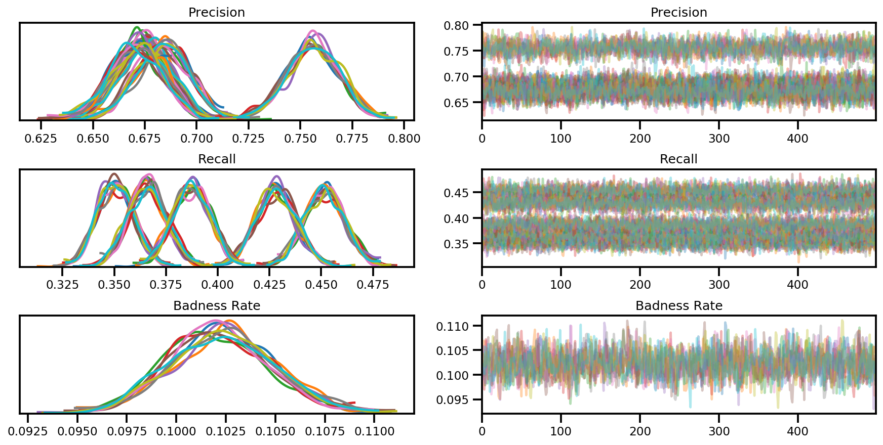
Inferenza (NUTS)
nchain = 10
prc, rcl, p_bad, _ = mdl_mixture.sample(nchain)
initial_chain_state = [prc, rcl, p_bad]

# Since MCMC operates over unconstrained space, we need to transform the
# samples so they live in real-space.
unconstraining_bijectors = [
    tfb.Sigmoid(),       # Maps R to [0, 1].
    tfb.Sigmoid(),       # Maps R to [0, 1].
    tfb.Sigmoid(),       # Maps R to [0, 1].
]
step_size = [tf.cast(i, dtype=dtype) for i in [1e-3, 1e-3, 1e-3]]

X_expanded = X_np[np.newaxis, ...]
target_log_prob_fn = lambda *x: mdl_mixture.log_prob(x + (X_expanded, ))

samples, sampler_stat = run_chain(
    initial_chain_state, step_size, target_log_prob_fn,
    unconstraining_bijectors, burnin=100)
# using the pymc3 naming convention
sample_stats_name = ['lp', 'tree_size', 'diverging', 'energy', 'mean_tree_accept']
sample_stats = {k:v.numpy().T for k, v in zip(sample_stats_name, sampler_stat)}
sample_stats['tree_size'] = np.diff(sample_stats['tree_size'], axis=1)

var_name = ['Precision', 'Recall', 'Badness Rate']
posterior = {k:np.swapaxes(v.numpy(), 1, 0)
             for k, v in zip(var_name, samples)}

az_trace = az.from_dict(posterior=posterior, sample_stats=sample_stats)
axes = az.plot_trace(az_trace, compact=True);