| | |  צפה במקור ב-GitHub צפה במקור ב-GitHub |
JointDistributionSequential היא הפצה דמוית חדש הציגה מח' שמשתמש מסמיך את המודל בייס אב טיפוס מהיר. זה מאפשר לך לשרשר הפצות מרובות יחד, ולהשתמש בפונקציית lambda כדי להציג תלות. זה נועד לבנות דגמים בייסיאניים קטנים עד בינוניים, כולל דגמים רבים בשימוש כמו GLMs, דגמי אפקט מעורב, דגמי תערובת ועוד. זה מאפשר את כל התכונות הדרושות עבור זרימת עבודה בייסיאנית: דגימה חזויה קודמת, זה יכול להיות תוסף למודל גרפי בייסיאני גדול אחר או לרשת עצבית. בשנת Colab זה, נוכל להראות כמה דוגמאות כיצד להשתמש JointDistributionSequential להשיג היום שלך כדי עבודה בייס יום
תלות ותנאים מוקדמים
# We will be using ArviZ, a multi-backend Bayesian diagnosis and plotting librarypip3 install -q git+git://github.com/arviz-devs/arviz.git
ייבוא והגדרות
from pprint import pprint
import matplotlib.pyplot as plt
import numpy as np
import seaborn as sns
import pandas as pd
import arviz as az

import tensorflow.compat.v2 as tf
tf.enable_v2_behavior()

import tensorflow_probability as tfp

sns.reset_defaults()
#sns.set_style('whitegrid')
#sns.set_context('talk')
sns.set_context(context='talk',font_scale=0.7)

%config InlineBackend.figure_format = 'retina'
%matplotlib inline

tfd = tfp.distributions
tfb = tfp.bijectors

dtype = tf.float64
הפוך דברים מהר!
לפני שנצלול פנימה, בואו נוודא שאנחנו משתמשים ב-GPU עבור הדגמה זו.
כדי לעשות זאת, בחר "זמן ריצה" -> "שנה סוג זמן ריצה" -> "מאיץ חומרה" -> "GPU".
הקטע הבא יאמת שיש לנו גישה ל-GPU.
if tf.test.gpu_device_name() != '/device:GPU:0':
  print('WARNING: GPU device not found.')
else:
  print('SUCCESS: Found GPU: {}'.format(tf.test.gpu_device_name()))
SUCCESS: Found GPU: /device:GPU:0
הפצה משותפת
הערות: שיעור הפצה זה שימושי כאשר יש לך רק מודל פשוט. "פשוט" פירושו גרפים דמויי שרשרת; למרות שהגישה טכנית עובדת עבור כל PGM עם תואר לכל היותר 255 עבור צומת בודד (מכיוון שלפונקציות Python יכולות להיות לכל היותר כל כך הרבה args).
הרעיון הבסיסי הוא שיש למשתמש לציין רשימת callable ים אשר מייצרים tfp.Distribution מקרים, אחד עבור כל קודקוד ב שלהם PGM . callable תהיה לכל היותר כמו ויכוחים רבים ככל האינדקס שלו ברשימה. (לנוחות המשתמש, אגומנטים יועברו בסדר הפוך של יצירה.) פנימית "נלך על הגרף" פשוט על ידי העברת ערך של כל RV קודם לכל אחד שניתן להתקשר. בעשותנו כך אנו ליישם את [חוק השרשרת של הסתברות] (https://en.wikipedia.org/wiki/Chain הכלל (% הסתברות 29 # More_than_two_random_variables): \(p(\{x\}_i^d)=\prod_i^d p(x_i|x_{<i})\).
הרעיון די פשוט, אפילו כקוד Python. הנה התמצית:
# The chain rule of probability, manifest as Python code.
def log_prob(rvs, xs):
  # xs[:i] is rv[i]'s markov blanket. `[::-1]` just reverses the list.
  return sum(rv(*xs[i-1::-1]).log_prob(xs[i])
             for i, rv in enumerate(rvs))
אתה יכול למצוא מידע נוסף מן docstring של JointDistributionSequential , אבל העיקר הוא שאתה עובר רשימה של הפצות כדי לאתחל את הכיתה, אם הפצות כמה ברשימה הוא תלוי פלט אחר הפצה / משתנה במעלה זרם, אתה פשוט לעטוף אותו עם פונקציית למבדה. עכשיו בואו נראה איך זה עובד בפעולה!
(חזק) רגרסיה לינארית
מתוך מסמך PyMC3 GLM: רגרסיה חזק עם איתור Outlier
קבל נתונים
dfhogg = pd.DataFrame(np.array([[1, 201, 592, 61, 9, -0.84],
[2, 244, 401, 25, 4, 0.31],
[3, 47, 583, 38, 11, 0.64],
[4, 287, 402, 15, 7, -0.27],
[5, 203, 495, 21, 5, -0.33],
[6, 58, 173, 15, 9, 0.67],
[7, 210, 479, 27, 4, -0.02],
[8, 202, 504, 14, 4, -0.05],
[9, 198, 510, 30, 11, -0.84],
[10, 158, 416, 16, 7, -0.69],
[11, 165, 393, 14, 5, 0.30],
[12, 201, 442, 25, 5, -0.46],
[13, 157, 317, 52, 5, -0.03],
[14, 131, 311, 16, 6, 0.50],
[15, 166, 400, 34, 6, 0.73],
[16, 160, 337, 31, 5, -0.52],
[17, 186, 423, 42, 9, 0.90],
[18, 125, 334, 26, 8, 0.40],
[19, 218, 533, 16, 6, -0.78],
[20, 146, 344, 22, 5, -0.56]]),
columns=['id','x','y','sigma_y','sigma_x','rho_xy'])
## for convenience zero-base the 'id' and use as index
dfhogg['id'] = dfhogg['id'] - 1
dfhogg.set_index('id', inplace=True)
## standardize (mean center and divide by 1 sd)
dfhoggs = (dfhogg[['x','y']] - dfhogg[['x','y']].mean(0)) / dfhogg[['x','y']].std(0)
dfhoggs['sigma_y'] = dfhogg['sigma_y'] / dfhogg['y'].std(0)
dfhoggs['sigma_x'] = dfhogg['sigma_x'] / dfhogg['x'].std(0)
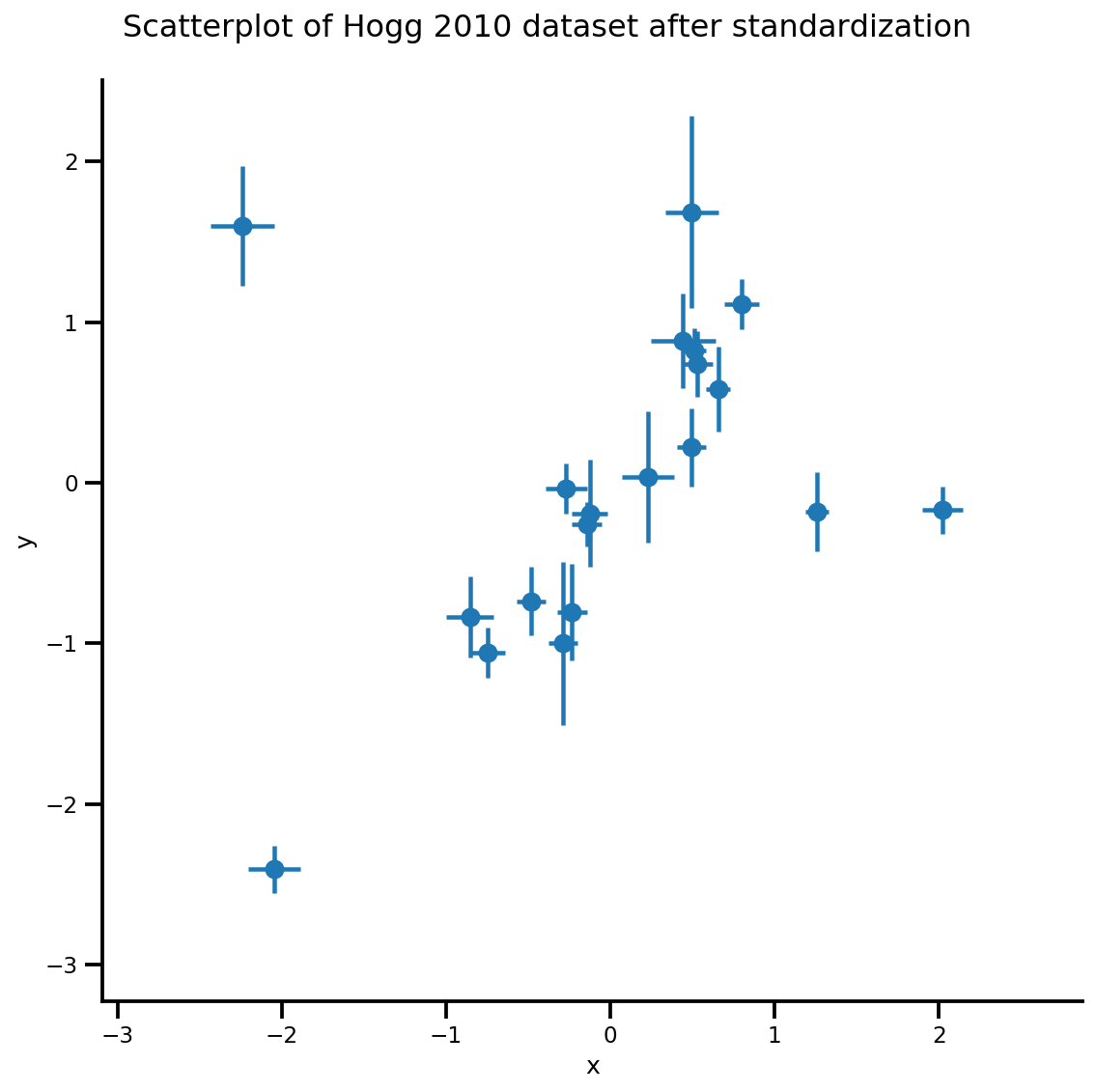
def plot_hoggs(dfhoggs):
## create xlims ylims for plotting
xlims = (dfhoggs['x'].min() - np.ptp(dfhoggs['x'])/5,
dfhoggs['x'].max() + np.ptp(dfhoggs['x'])/5)
ylims = (dfhoggs['y'].min() - np.ptp(dfhoggs['y'])/5,
dfhoggs['y'].max() + np.ptp(dfhoggs['y'])/5)
## scatterplot the standardized data
g = sns.FacetGrid(dfhoggs, size=8)
_ = g.map(plt.errorbar, 'x', 'y', 'sigma_y', 'sigma_x', marker="o", ls='')
_ = g.axes[0][0].set_ylim(ylims)
_ = g.axes[0][0].set_xlim(xlims)
plt.subplots_adjust(top=0.92)
_ = g.fig.suptitle('Scatterplot of Hogg 2010 dataset after standardization', fontsize=16)
return g, xlims, ylims
g = plot_hoggs(dfhoggs)
/usr/local/lib/python3.6/dist-packages/numpy/core/fromnumeric.py:2495: FutureWarning: Method .ptp is deprecated and will be removed in a future version. Use numpy.ptp instead.
  return ptp(axis=axis, out=out, **kwargs)
/usr/local/lib/python3.6/dist-packages/seaborn/axisgrid.py:230: UserWarning: The `size` paramter has been renamed to `height`; please update your code.
  warnings.warn(msg, UserWarning)
X_np = dfhoggs['x'].values
sigma_y_np = dfhoggs['sigma_y'].values
Y_np = dfhoggs['y'].values
דגם OLS קונבנציונלי
כעת, בואו נגדיר מודל ליניארי, בעיה פשוטה של יירוט + רגרסיה של שיפוע:
mdl_ols = tfd.JointDistributionSequential([
    # b0 ~ Normal(0, 1)
    tfd.Normal(loc=tf.cast(0, dtype), scale=1.),
    # b1 ~ Normal(0, 1)
    tfd.Normal(loc=tf.cast(0, dtype), scale=1.),
    # x ~ Normal(b0+b1*X, 1)
    lambda b1, b0: tfd.Normal(
      # Parameter transformation
      loc=b0 + b1*X_np,
      scale=sigma_y_np)
])
לאחר מכן תוכל לבדוק את הגרף של המודל כדי לראות את התלות. שים לב x שמורה כמו השם של הצומת האחרונה, ואתה לא יכול להבטיח את זה בתור הטיעון למבדה שלך במודל JointDistributionSequential שלך.
mdl_ols.resolve_graph()
(('b0', ()), ('b1', ()), ('x', ('b1', 'b0')))
הדגימה מהדגם היא די פשוטה:
mdl_ols.sample()
[<tf.Tensor: shape=(), dtype=float64, numpy=-0.50225804634794>,
 <tf.Tensor: shape=(), dtype=float64, numpy=0.682740126293564>,
 <tf.Tensor: shape=(20,), dtype=float64, numpy=
 array([-0.33051382,  0.71443618, -1.91085683,  0.89371173, -0.45060957,
        -1.80448758, -0.21357082,  0.07891058, -0.20689721, -0.62690385,
        -0.55225748, -0.11446535, -0.66624497, -0.86913291, -0.93605552,
        -0.83965336, -0.70988597, -0.95813437,  0.15884761, -0.31113434])>]
...אשר נותן רשימה של tf.Tensor. אתה יכול לחבר אותו מיד לפונקציה log_prob כדי לחשב את log_prob של המודל:
prior_predictive_samples = mdl_ols.sample()
mdl_ols.log_prob(prior_predictive_samples)
<tf.Tensor: shape=(20,), dtype=float64, numpy=
array([-4.97502846, -3.98544303, -4.37514505, -3.46933487, -3.80688125,
       -3.42907525, -4.03263074, -3.3646366 , -4.70370938, -4.36178501,
       -3.47823735, -3.94641662, -5.76906319, -4.0944128 , -4.39310708,
       -4.47713894, -4.46307881, -3.98802372, -3.83027747, -4.64777082])>
הממ, משהו כאן לא בסדר: אנחנו אמורים לקבל log_prob סקלארי! למעשה, אנחנו עוד יכולים לבדוק אם משהו כבוי על ידי קריאת .log_prob_parts , אשר נותן את log_prob של כול צומת במודל הגרפי:
mdl_ols.log_prob_parts(prior_predictive_samples)
[<tf.Tensor: shape=(), dtype=float64, numpy=-0.9699239562734849>,
 <tf.Tensor: shape=(), dtype=float64, numpy=-3.459364167569284>,
 <tf.Tensor: shape=(20,), dtype=float64, numpy=
 array([-0.54574034,  0.4438451 ,  0.05414307,  0.95995326,  0.62240687,
         1.00021288,  0.39665739,  1.06465152, -0.27442125,  0.06750311,
         0.95105078,  0.4828715 , -1.33977506,  0.33487533,  0.03618104,
        -0.04785082, -0.03379069,  0.4412644 ,  0.59901066, -0.2184827 ])>]
... מסתבר שהצומת האחרון אינו מוחל ב-reduc_sum לאורך הממד/ציר iid! כאשר אנו עושים את הסכום, שני המשתנים הראשונים משודרים בצורה שגויה.
הטריק כאן הוא להשתמש tfd.Independent כדי פרש את הצורה יצווה (כך שאר הציר יופחת בצורה נכונה):
mdl_ols_ = tfd.JointDistributionSequential([
    # b0
    tfd.Normal(loc=tf.cast(0, dtype), scale=1.),
    # b1
    tfd.Normal(loc=tf.cast(0, dtype), scale=1.),
    # likelihood
    #   Using Independent to ensure the log_prob is not incorrectly broadcasted
    lambda b1, b0: tfd.Independent(
        tfd.Normal(
            # Parameter transformation
            # b1 shape: (batch_shape), X shape (num_obs): we want result to have
            # shape (batch_shape, num_obs)
            loc=b0 + b1*X_np,
            scale=sigma_y_np),
        reinterpreted_batch_ndims=1
    ),
])
כעת, בוא נבדוק את הצומת/הפצה האחרונה של המודל, אתה יכול לראות שצורת האירוע מתפרשת נכון. הערה כי זה עלול לקחת קצת ניסוי וטעייה כדי לקבל את reinterpreted_batch_ndims תקין, אבל אתה תמיד יכול בקלות להדפיס את ההפצה או מותח שנדגמו כדי לבדוק פעמיים את הצורה!
print(mdl_ols_.sample_distributions()[0][-1])
print(mdl_ols.sample_distributions()[0][-1])
tfp.distributions.Independent("JointDistributionSequential_sample_distributions_IndependentJointDistributionSequential_sample_distributions_Normal", batch_shape=[], event_shape=[20], dtype=float64)
tfp.distributions.Normal("JointDistributionSequential_sample_distributions_Normal", batch_shape=[20], event_shape=[], dtype=float64)
prior_predictive_samples = mdl_ols_.sample()
mdl_ols_.log_prob(prior_predictive_samples)  # <== Getting a scalar correctly
<tf.Tensor: shape=(), dtype=float64, numpy=-2.543425661013286>
אחרים JointDistribution* API
mdl_ols_named = tfd.JointDistributionNamed(dict(
    likelihood = lambda b0, b1: tfd.Independent(
        tfd.Normal(
            loc=b0 + b1*X_np,
            scale=sigma_y_np),
        reinterpreted_batch_ndims=1
    ),
    b0         = tfd.Normal(loc=tf.cast(0, dtype), scale=1.),
    b1         = tfd.Normal(loc=tf.cast(0, dtype), scale=1.),
))

mdl_ols_named.log_prob(mdl_ols_named.sample())
<tf.Tensor: shape=(), dtype=float64, numpy=-5.99620966071338>
mdl_ols_named.sample() # output is a dictionary
{'b0': <tf.Tensor: shape=(), dtype=float64, numpy=0.26364058399428225>,
 'b1': <tf.Tensor: shape=(), dtype=float64, numpy=-0.27209402374432207>,
 'likelihood': <tf.Tensor: shape=(20,), dtype=float64, numpy=
 array([ 0.6482155 , -0.39314108,  0.62744764, -0.24587987, -0.20544617,
         1.01465392, -0.04705611, -0.16618702,  0.36410134,  0.3943299 ,
         0.36455291, -0.27822219, -0.24423928,  0.24599518,  0.82731092,
        -0.21983033,  0.56753169,  0.32830481, -0.15713064,  0.23336351])>}
Root = tfd.JointDistributionCoroutine.Root  # Convenient alias.
def model():
  b1 = yield Root(tfd.Normal(loc=tf.cast(0, dtype), scale=1.))
  b0 = yield Root(tfd.Normal(loc=tf.cast(0, dtype), scale=1.))
  yhat = b0 + b1*X_np
  likelihood = yield tfd.Independent(
        tfd.Normal(loc=yhat, scale=sigma_y_np),
        reinterpreted_batch_ndims=1
    )

mdl_ols_coroutine = tfd.JointDistributionCoroutine(model)
mdl_ols_coroutine.log_prob(mdl_ols_coroutine.sample())
<tf.Tensor: shape=(), dtype=float64, numpy=-4.566678123520463>
mdl_ols_coroutine.sample() # output is a tuple
(<tf.Tensor: shape=(), dtype=float64, numpy=0.06811002171170354>,
 <tf.Tensor: shape=(), dtype=float64, numpy=-0.37477064754116807>,
 <tf.Tensor: shape=(20,), dtype=float64, numpy=
 array([-0.91615096, -0.20244718, -0.47840159, -0.26632479, -0.60441105,
        -0.48977789, -0.32422329, -0.44019322, -0.17072643, -0.20666025,
        -0.55932191, -0.40801868, -0.66893181, -0.24134135, -0.50403536,
        -0.51788596, -0.90071876, -0.47382338, -0.34821655, -0.38559724])>)
MLE
ועכשיו אנחנו יכולים לעשות מסקנות! אתה יכול להשתמש באופטימיזציה כדי למצוא את אומדן הסבירות המקסימלית.
הגדר כמה פונקציות עוזר
# bfgs and lbfgs currently requries a function that returns both the value and
# gradient re the input.
import functools

def _make_val_and_grad_fn(value_fn):
  @functools.wraps(value_fn)
  def val_and_grad(x):
    return tfp.math.value_and_gradient(value_fn, x)
  return val_and_grad

# Map a list of tensors (e.g., output from JDSeq.sample([...])) to a single tensor
# modify from tfd.Blockwise
from tensorflow_probability.python.internal import dtype_util
from tensorflow_probability.python.internal import prefer_static as ps
from tensorflow_probability.python.internal import tensorshape_util

class Mapper:
  """Basically, this is a bijector without log-jacobian correction."""
  def __init__(self, list_of_tensors, list_of_bijectors, event_shape):
    self.dtype = dtype_util.common_dtype(
        list_of_tensors, dtype_hint=tf.float32)
    self.list_of_tensors = list_of_tensors
    self.bijectors = list_of_bijectors
    self.event_shape = event_shape

  def flatten_and_concat(self, list_of_tensors):
    def _reshape_map_part(part, event_shape, bijector):
      part = tf.cast(bijector.inverse(part), self.dtype)
      static_rank = tf.get_static_value(ps.rank_from_shape(event_shape))
      if static_rank == 1:
        return part
      new_shape = ps.concat([
          ps.shape(part)[:ps.size(ps.shape(part)) - ps.size(event_shape)],
          [-1]
      ], axis=-1)
      return tf.reshape(part, ps.cast(new_shape, tf.int32))

    x = tf.nest.map_structure(_reshape_map_part,
                              list_of_tensors,
                              self.event_shape,
                              self.bijectors)
    return tf.concat(tf.nest.flatten(x), axis=-1)

  def split_and_reshape(self, x):
    assertions = []
    message = 'Input must have at least one dimension.'
    if tensorshape_util.rank(x.shape) is not None:
      if tensorshape_util.rank(x.shape) == 0:
        raise ValueError(message)
    else:
      assertions.append(assert_util.assert_rank_at_least(x, 1, message=message))
    with tf.control_dependencies(assertions):
      splits = [
          tf.cast(ps.maximum(1, ps.reduce_prod(s)), tf.int32)
          for s in tf.nest.flatten(self.event_shape)
      ]
      x = tf.nest.pack_sequence_as(
          self.event_shape, tf.split(x, splits, axis=-1))
      def _reshape_map_part(part, part_org, event_shape, bijector):
        part = tf.cast(bijector.forward(part), part_org.dtype)
        static_rank = tf.get_static_value(ps.rank_from_shape(event_shape))
        if static_rank == 1:
          return part
        new_shape = ps.concat([ps.shape(part)[:-1], event_shape], axis=-1)
        return tf.reshape(part, ps.cast(new_shape, tf.int32))

      x = tf.nest.map_structure(_reshape_map_part,
                                x,
                                self.list_of_tensors,
                                self.event_shape,
                                self.bijectors)
    return x
mapper = Mapper(mdl_ols_.sample()[:-1],
                [tfb.Identity(), tfb.Identity()],
                mdl_ols_.event_shape[:-1])

# mapper.split_and_reshape(mapper.flatten_and_concat(mdl_ols_.sample()[:-1]))
@_make_val_and_grad_fn
def neg_log_likelihood(x):
  # Generate a function closure so that we are computing the log_prob
  # conditioned on the observed data. Note also that tfp.optimizer.* takes a
  # single tensor as input.
  return -mdl_ols_.log_prob(mapper.split_and_reshape(x) + [Y_np])

lbfgs_results = tfp.optimizer.lbfgs_minimize(
    neg_log_likelihood,
    initial_position=tf.zeros(2, dtype=dtype),
    tolerance=1e-20,
    x_tolerance=1e-8
)
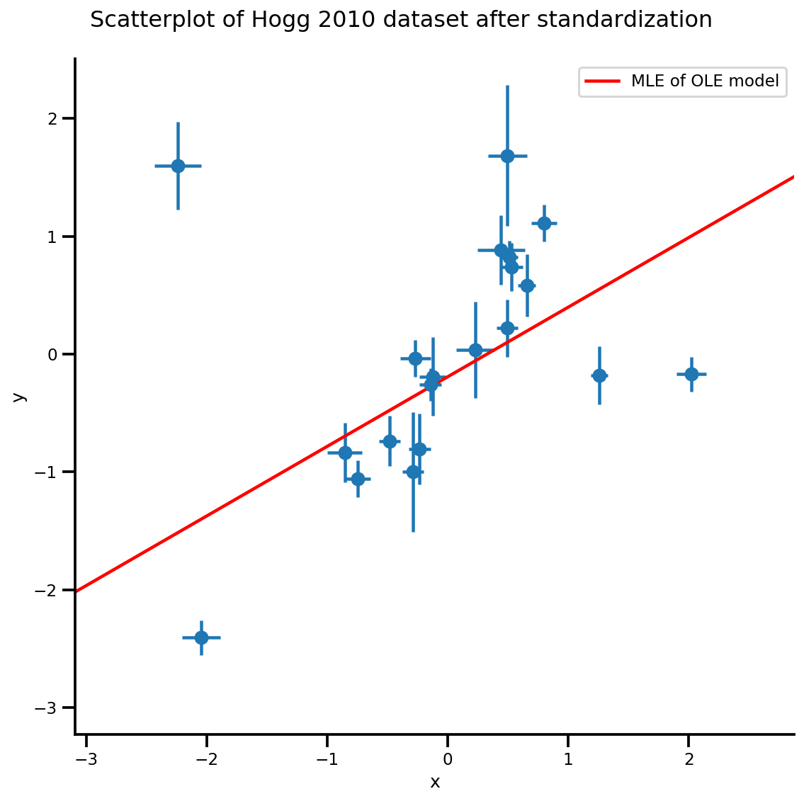
b0est, b1est = lbfgs_results.position.numpy()

g, xlims, ylims = plot_hoggs(dfhoggs);
xrange = np.linspace(xlims[0], xlims[1], 100)
g.axes[0][0].plot(xrange, b0est + b1est*xrange,
                  color='r', label='MLE of OLE model')
plt.legend();
/usr/local/lib/python3.6/dist-packages/numpy/core/fromnumeric.py:2495: FutureWarning: Method .ptp is deprecated and will be removed in a future version. Use numpy.ptp instead.
  return ptp(axis=axis, out=out, **kwargs)
/usr/local/lib/python3.6/dist-packages/seaborn/axisgrid.py:230: UserWarning: The `size` paramter has been renamed to `height`; please update your code.
  warnings.warn(msg, UserWarning)
דגם גרסת אצווה ו-MCMC
בשנת הסקה בייס, אנחנו בדרך כלל רוצים לעבוד עם דגימות המרק"ם, כאשר הדגימות הן מן האחוריים, אנחנו יכולים לחבר אותם לתוך כל פונקציה לציפיות מחשוב. עם זאת, ה- API המרק"ם מחייב אותנו לכתוב דגמים כי הם יצוו ידידותיים, ואנחנו יכולים לבדוק כי המודל שלנו הוא בעצם לא "batchable" על ידי התקשרות sample([...])
mdl_ols_.sample(5) # <== error as some computation could not be broadcasted.
במקרה זה, זה יחסית פשוט מכיוון שיש לנו רק פונקציה לינארית בתוך המודל שלנו, הרחבת הצורה אמורה לעשות את העבודה:
mdl_ols_batch = tfd.JointDistributionSequential([
    # b0
    tfd.Normal(loc=tf.cast(0, dtype), scale=1.),
    # b1
    tfd.Normal(loc=tf.cast(0, dtype), scale=1.),
    # likelihood
    #   Using Independent to ensure the log_prob is not incorrectly broadcasted
    lambda b1, b0: tfd.Independent(
        tfd.Normal(
            # Parameter transformation
            loc=b0[..., tf.newaxis] + b1[..., tf.newaxis]*X_np[tf.newaxis, ...],
            scale=sigma_y_np[tf.newaxis, ...]),
        reinterpreted_batch_ndims=1
    ),
])

mdl_ols_batch.resolve_graph()
(('b0', ()), ('b1', ()), ('x', ('b1', 'b0')))
נוכל שוב לדגום ולהעריך את log_prob_parts כדי לבצע כמה בדיקות:
b0, b1, y = mdl_ols_batch.sample(4)
mdl_ols_batch.log_prob_parts([b0, b1, y])
[<tf.Tensor: shape=(4,), dtype=float64, numpy=array([-1.25230168, -1.45281432, -1.87110061, -1.07665206])>,
 <tf.Tensor: shape=(4,), dtype=float64, numpy=array([-1.07019936, -1.59562117, -2.53387765, -1.01557632])>,
 <tf.Tensor: shape=(4,), dtype=float64, numpy=array([ 0.45841406,  2.56829635, -4.84973951, -5.59423992])>]
כמה הערות צדדיות:
- אנחנו רוצים לעבוד עם גרסת אצווה של הדגם מכיוון שהיא המהירה ביותר עבור MCMC מרובה שרשרת. במקרים שלא ניתן לשכתב את המודל כגרסת באצוות (למשל, מודלים אודה), אתה יכול למפות את פונקצית log_prob באמצעות
tf.map_fnכדי להשיג את אותו האפקט. - עכשיו
mdl_ols_batch.sample()אולי לא עבודה כמו שיש לנו scaler לפני, כמו שאנחנו לא יכולים לעשותscaler_tensor[:, None]. הפתרון כאן היא להרחיב מותח scaler כדי דרגה 1 על ידי גלישתtfd.Sample(..., sample_shape=1). - זה תרגול טוב לכתוב את המודל כפונקציה כדי שתוכל לשנות הגדרות כמו היפרפרמטרים הרבה יותר קל.
def gen_ols_batch_model(X, sigma, hyperprior_mean=0, hyperprior_scale=1):
  hyper_mean = tf.cast(hyperprior_mean, dtype)
  hyper_scale = tf.cast(hyperprior_scale, dtype)
  return tfd.JointDistributionSequential([
      # b0
      tfd.Sample(tfd.Normal(loc=hyper_mean, scale=hyper_scale), sample_shape=1),
      # b1
      tfd.Sample(tfd.Normal(loc=hyper_mean, scale=hyper_scale), sample_shape=1),
      # likelihood
      lambda b1, b0: tfd.Independent(
          tfd.Normal(
              # Parameter transformation
              loc=b0 + b1*X,
              scale=sigma),
          reinterpreted_batch_ndims=1
      ),
  ], validate_args=True)

mdl_ols_batch = gen_ols_batch_model(X_np[tf.newaxis, ...],
                                    sigma_y_np[tf.newaxis, ...])

_ = mdl_ols_batch.sample()
_ = mdl_ols_batch.sample(4)
_ = mdl_ols_batch.sample([3, 4])
# Small helper function to validate log_prob shape (avoid wrong broadcasting)
def validate_log_prob_part(model, batch_shape=1, observed=-1):
  samples = model.sample(batch_shape)
  logp_part = list(model.log_prob_parts(samples))

  # exclude observed node
  logp_part.pop(observed)
  for part in logp_part:
    tf.assert_equal(part.shape, logp_part[-1].shape)

validate_log_prob_part(mdl_ols_batch, 4)
בדיקות נוספות: השוואת פונקציית log_prob שנוצרה עם פונקציית TFP log_prob בכתב יד.
def ols_logp_batch(b0, b1, Y):
  b0_prior = tfd.Normal(loc=tf.cast(0, dtype), scale=1.) # b0
  b1_prior = tfd.Normal(loc=tf.cast(0, dtype), scale=1.) # b1
  likelihood = tfd.Normal(loc=b0 + b1*X_np[None, :],
                          scale=sigma_y_np) # likelihood
  return tf.reduce_sum(b0_prior.log_prob(b0), axis=-1) +\
         tf.reduce_sum(b1_prior.log_prob(b1), axis=-1) +\
         tf.reduce_sum(likelihood.log_prob(Y), axis=-1)

b0, b1, x = mdl_ols_batch.sample(4)
print(mdl_ols_batch.log_prob([b0, b1, Y_np]).numpy())
print(ols_logp_batch(b0, b1, Y_np).numpy())
[-227.37899384 -327.10043743 -570.44162789 -702.79808683]
[-227.37899384 -327.10043743 -570.44162789 -702.79808683]
MCMC באמצעות ה-No-Turn Sampler
נפוצה run_chain פונקציה
@tf.function(autograph=False, experimental_compile=True)
def run_chain(init_state, step_size, target_log_prob_fn, unconstraining_bijectors,
              num_steps=500, burnin=50):

  def trace_fn(_, pkr):
    return (
        pkr.inner_results.inner_results.target_log_prob,
        pkr.inner_results.inner_results.leapfrogs_taken,
        pkr.inner_results.inner_results.has_divergence,
        pkr.inner_results.inner_results.energy,
        pkr.inner_results.inner_results.log_accept_ratio
           )

  kernel = tfp.mcmc.TransformedTransitionKernel(
    inner_kernel=tfp.mcmc.NoUTurnSampler(
      target_log_prob_fn,
      step_size=step_size),
    bijector=unconstraining_bijectors)

  hmc = tfp.mcmc.DualAveragingStepSizeAdaptation(
    inner_kernel=kernel,
    num_adaptation_steps=burnin,
    step_size_setter_fn=lambda pkr, new_step_size: pkr._replace(
        inner_results=pkr.inner_results._replace(step_size=new_step_size)),
    step_size_getter_fn=lambda pkr: pkr.inner_results.step_size,
    log_accept_prob_getter_fn=lambda pkr: pkr.inner_results.log_accept_ratio
  )

  # Sampling from the chain.
  chain_state, sampler_stat = tfp.mcmc.sample_chain(
      num_results=num_steps,
      num_burnin_steps=burnin,
      current_state=init_state,
      kernel=hmc,
      trace_fn=trace_fn)
  return chain_state, sampler_stat
nchain = 10
b0, b1, _ = mdl_ols_batch.sample(nchain)
init_state = [b0, b1]
step_size = [tf.cast(i, dtype=dtype) for i in [.1, .1]]
target_log_prob_fn = lambda *x: mdl_ols_batch.log_prob(x + (Y_np, ))

# bijector to map contrained parameters to real
unconstraining_bijectors = [
    tfb.Identity(),
    tfb.Identity(),
]

samples, sampler_stat = run_chain(
    init_state, step_size, target_log_prob_fn, unconstraining_bijectors)
# using the pymc3 naming convention
sample_stats_name = ['lp', 'tree_size', 'diverging', 'energy', 'mean_tree_accept']
sample_stats = {k:v.numpy().T for k, v in zip(sample_stats_name, sampler_stat)}
sample_stats['tree_size'] = np.diff(sample_stats['tree_size'], axis=1)
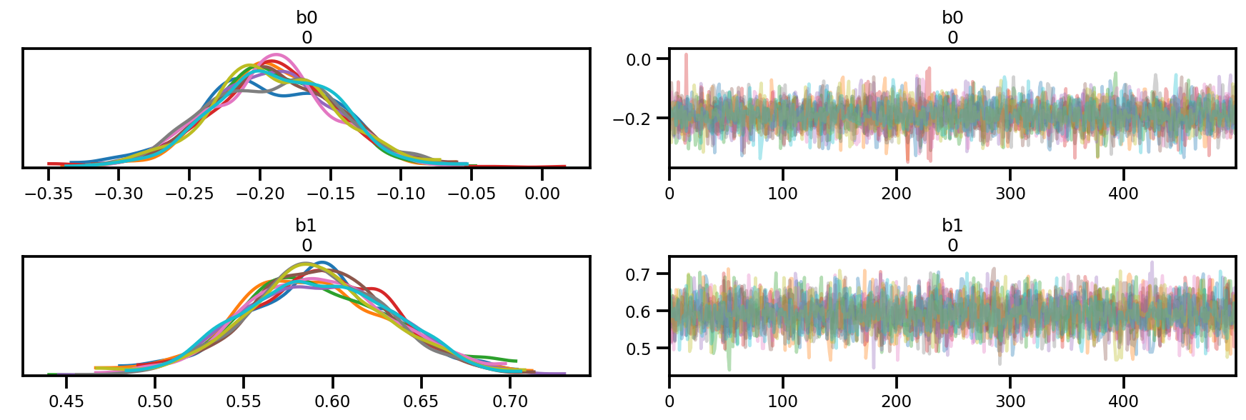
var_name = ['b0', 'b1']
posterior = {k:np.swapaxes(v.numpy(), 1, 0)
for k, v in zip(var_name, samples)}
az_trace = az.from_dict(posterior=posterior, sample_stats=sample_stats)
az.plot_trace(az_trace);
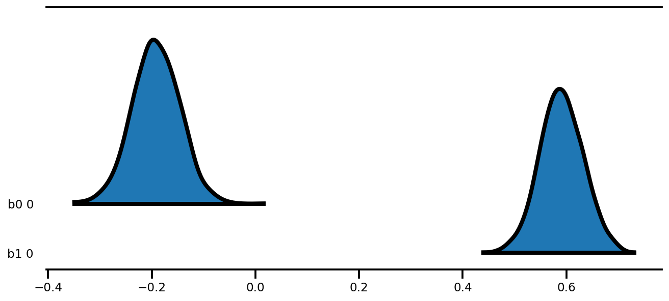
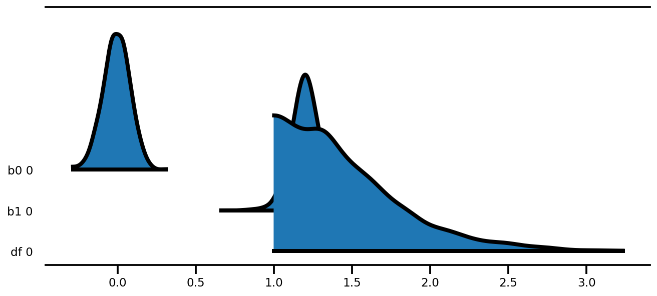
az.plot_forest(az_trace,
               kind='ridgeplot',
               linewidth=4,
               combined=True,
               ridgeplot_overlap=1.5,
               figsize=(9, 4));
k = 5
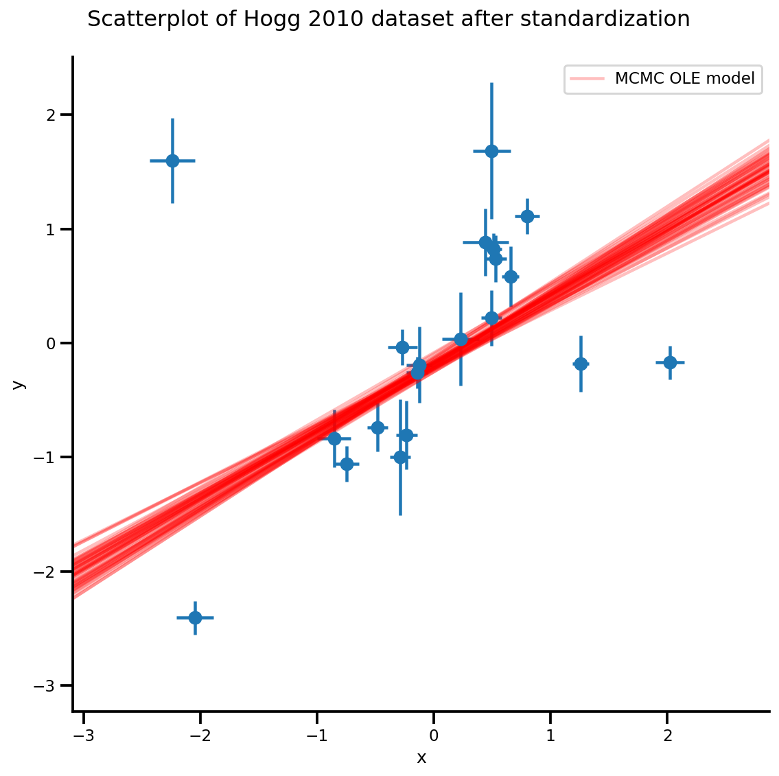
b0est, b1est = az_trace.posterior['b0'][:, -k:].values, az_trace.posterior['b1'][:, -k:].values
g, xlims, ylims = plot_hoggs(dfhoggs);
xrange = np.linspace(xlims[0], xlims[1], 100)[None, :]
g.axes[0][0].plot(np.tile(xrange, (k, 1)).T,
(np.reshape(b0est, [-1, 1]) + np.reshape(b1est, [-1, 1])*xrange).T,
alpha=.25, color='r')
plt.legend([g.axes[0][0].lines[-1]], ['MCMC OLE model']);
/usr/local/lib/python3.6/dist-packages/numpy/core/fromnumeric.py:2495: FutureWarning: Method .ptp is deprecated and will be removed in a future version. Use numpy.ptp instead.
  return ptp(axis=axis, out=out, **kwargs)
/usr/local/lib/python3.6/dist-packages/seaborn/axisgrid.py:230: UserWarning: The `size` paramter has been renamed to `height`; please update your code.
  warnings.warn(msg, UserWarning)
/usr/local/lib/python3.6/dist-packages/ipykernel_launcher.py:8: MatplotlibDeprecationWarning: cycling among columns of inputs with non-matching shapes is deprecated.
Student-T Method
שימו לב שמעכשיו אנחנו תמיד עובדים עם גרסת האצווה של דגם
def gen_studentt_model(X, sigma,
                       hyper_mean=0, hyper_scale=1, lower=1, upper=100):
  loc = tf.cast(hyper_mean, dtype)
  scale = tf.cast(hyper_scale, dtype)
  low = tf.cast(lower, dtype)
  high = tf.cast(upper, dtype)
  return tfd.JointDistributionSequential([
      # b0 ~ Normal(0, 1)
      tfd.Sample(tfd.Normal(loc, scale), sample_shape=1),
      # b1 ~ Normal(0, 1)
      tfd.Sample(tfd.Normal(loc, scale), sample_shape=1),
      # df ~ Uniform(a, b)
      tfd.Sample(tfd.Uniform(low, high), sample_shape=1),
      # likelihood ~ StudentT(df, f(b0, b1), sigma_y)
      #   Using Independent to ensure the log_prob is not incorrectly broadcasted.
      lambda df, b1, b0: tfd.Independent(
          tfd.StudentT(df=df, loc=b0 + b1*X, scale=sigma)),
  ], validate_args=True)

mdl_studentt = gen_studentt_model(X_np[tf.newaxis, ...],
                                  sigma_y_np[tf.newaxis, ...])
mdl_studentt.resolve_graph()
(('b0', ()), ('b1', ()), ('df', ()), ('x', ('df', 'b1', 'b0')))
validate_log_prob_part(mdl_studentt, 4)
דגימה קדימה (דגימה חזויה קודמת)
b0, b1, df, x = mdl_studentt.sample(1000)
x.shape
TensorShape([1000, 20])
MLE
# bijector to map contrained parameters to real
a, b = tf.constant(1., dtype), tf.constant(100., dtype),

# Interval transformation
tfp_interval = tfb.Inline(
    inverse_fn=(
        lambda x: tf.math.log(x - a) - tf.math.log(b - x)),
    forward_fn=(
        lambda y: (b - a) * tf.sigmoid(y) + a),
    forward_log_det_jacobian_fn=(
        lambda x: tf.math.log(b - a) - 2 * tf.nn.softplus(-x) - x),
    forward_min_event_ndims=0,
    name="interval")

unconstraining_bijectors = [
    tfb.Identity(),
    tfb.Identity(),
    tfp_interval,
]

mapper = Mapper(mdl_studentt.sample()[:-1],
                unconstraining_bijectors,
                mdl_studentt.event_shape[:-1])
@_make_val_and_grad_fn
def neg_log_likelihood(x):
  # Generate a function closure so that we are computing the log_prob
  # conditioned on the observed data. Note also that tfp.optimizer.* takes a
  # single tensor as input, so we need to do some slicing here:
  return -tf.squeeze(mdl_studentt.log_prob(
      mapper.split_and_reshape(x) + [Y_np]))

lbfgs_results = tfp.optimizer.lbfgs_minimize(
    neg_log_likelihood,
    initial_position=mapper.flatten_and_concat(mdl_studentt.sample()[:-1]),
    tolerance=1e-20,
    x_tolerance=1e-20
)
b0est, b1est, dfest = lbfgs_results.position.numpy()
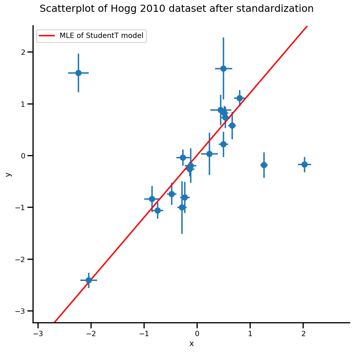
g, xlims, ylims = plot_hoggs(dfhoggs);
xrange = np.linspace(xlims[0], xlims[1], 100)
g.axes[0][0].plot(xrange, b0est + b1est*xrange,
color='r', label='MLE of StudentT model')
plt.legend();
/usr/local/lib/python3.6/dist-packages/numpy/core/fromnumeric.py:2495: FutureWarning: Method .ptp is deprecated and will be removed in a future version. Use numpy.ptp instead.
  return ptp(axis=axis, out=out, **kwargs)
/usr/local/lib/python3.6/dist-packages/seaborn/axisgrid.py:230: UserWarning: The `size` paramter has been renamed to `height`; please update your code.
  warnings.warn(msg, UserWarning)
MCMC
nchain = 10
b0, b1, df, _ = mdl_studentt.sample(nchain)
init_state = [b0, b1, df]
step_size = [tf.cast(i, dtype=dtype) for i in [.1, .1, .05]]

target_log_prob_fn = lambda *x: mdl_studentt.log_prob(x + (Y_np, ))

samples, sampler_stat = run_chain(
    init_state, step_size, target_log_prob_fn, unconstraining_bijectors, burnin=100)
# using the pymc3 naming convention
sample_stats_name = ['lp', 'tree_size', 'diverging', 'energy', 'mean_tree_accept']
sample_stats = {k:v.numpy().T for k, v in zip(sample_stats_name, sampler_stat)}
sample_stats['tree_size'] = np.diff(sample_stats['tree_size'], axis=1)
var_name = ['b0', 'b1', 'df']
posterior = {k:np.swapaxes(v.numpy(), 1, 0)
for k, v in zip(var_name, samples)}
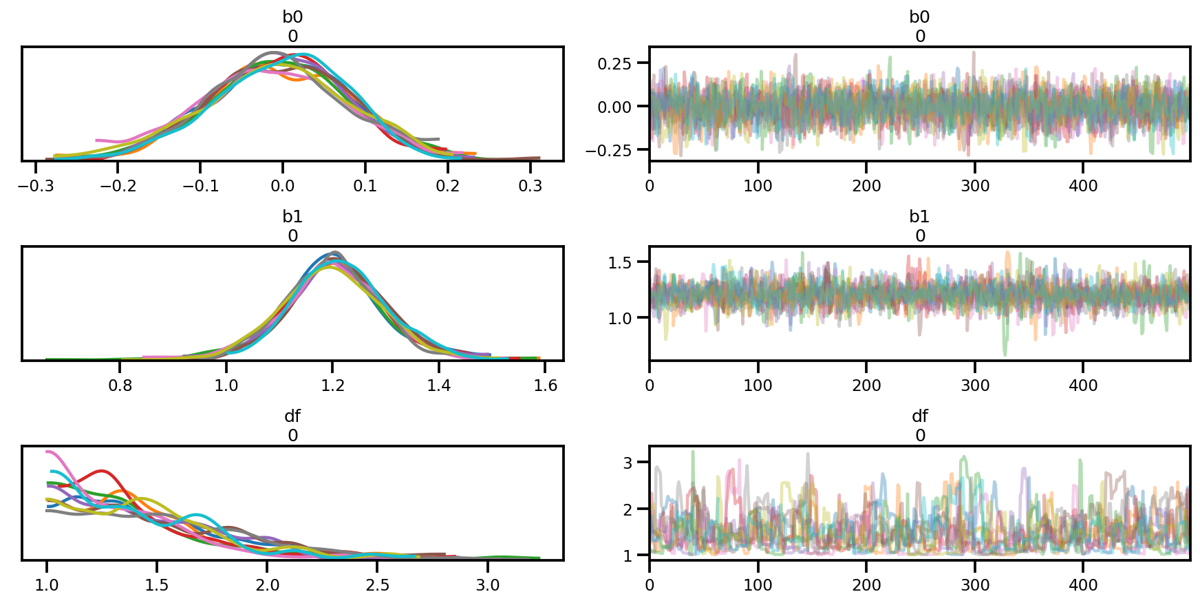
az_trace = az.from_dict(posterior=posterior, sample_stats=sample_stats)
az.summary(az_trace)
az.plot_trace(az_trace);
az.plot_forest(az_trace,
               kind='ridgeplot',
               linewidth=4,
               combined=True,
               ridgeplot_overlap=1.5,
               figsize=(9, 4));
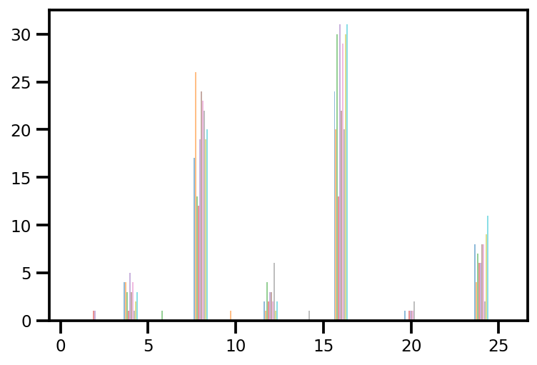
plt.hist(az_trace.sample_stats['tree_size'], np.linspace(.5, 25.5, 26), alpha=.5);
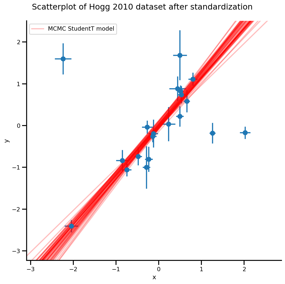
k = 5
b0est, b1est = az_trace.posterior['b0'][:, -k:].values, az_trace.posterior['b1'][:, -k:].values

g, xlims, ylims = plot_hoggs(dfhoggs);
xrange = np.linspace(xlims[0], xlims[1], 100)[None, :]
g.axes[0][0].plot(np.tile(xrange, (k, 1)).T,
                  (np.reshape(b0est, [-1, 1]) + np.reshape(b1est, [-1, 1])*xrange).T,
                  alpha=.25, color='r')
plt.legend([g.axes[0][0].lines[-1]], ['MCMC StudentT model']);
/usr/local/lib/python3.6/dist-packages/numpy/core/fromnumeric.py:2495: FutureWarning: Method .ptp is deprecated and will be removed in a future version. Use numpy.ptp instead.
  return ptp(axis=axis, out=out, **kwargs)
/usr/local/lib/python3.6/dist-packages/seaborn/axisgrid.py:230: UserWarning: The `size` paramter has been renamed to `height`; please update your code.
  warnings.warn(msg, UserWarning)
/usr/local/lib/python3.6/dist-packages/ipykernel_launcher.py:8: MatplotlibDeprecationWarning: cycling among columns of inputs with non-matching shapes is deprecated.
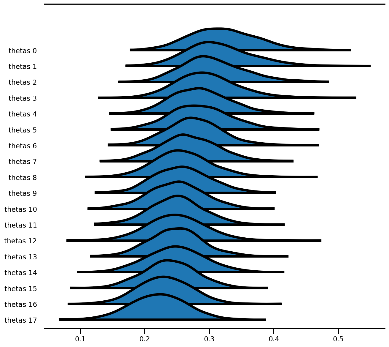
איגוד חלקי היררכי
מ PyMC3 נתוני בייסבול עבור 18 שחקנים מ אפרון מוריס (1975)
data = pd.read_table('https://raw.githubusercontent.com/pymc-devs/pymc3/master/pymc3/examples/data/efron-morris-75-data.tsv',
                     sep="\t")
at_bats, hits = data[['At-Bats', 'Hits']].values.T
n = len(at_bats)
def gen_baseball_model(at_bats, rate=1.5, a=0, b=1):
  return tfd.JointDistributionSequential([
    # phi
    tfd.Uniform(low=tf.cast(a, dtype), high=tf.cast(b, dtype)),
    # kappa_log
    tfd.Exponential(rate=tf.cast(rate, dtype)),
    # thetas
    lambda kappa_log, phi: tfd.Sample(
        tfd.Beta(
            concentration1=tf.exp(kappa_log)*phi,
            concentration0=tf.exp(kappa_log)*(1.0-phi)),
        sample_shape=n
    ),
    # likelihood
    lambda thetas: tfd.Independent(
        tfd.Binomial(
            total_count=tf.cast(at_bats, dtype),
            probs=thetas
        )),
])

mdl_baseball = gen_baseball_model(at_bats)
mdl_baseball.resolve_graph()
(('phi', ()),
 ('kappa_log', ()),
 ('thetas', ('kappa_log', 'phi')),
 ('x', ('thetas',)))
דגימה קדימה (דגימה חזויה קודמת)
phi, kappa_log, thetas, y = mdl_baseball.sample(4)
# phi, kappa_log, thetas, y
שוב, שימו לב כיצד אם לא תשתמשו ב-Independent, תקבלו log_prob שיש לו batch_shape שגוי.
# check logp
pprint(mdl_baseball.log_prob_parts([phi, kappa_log, thetas, hits]))
print(mdl_baseball.log_prob([phi, kappa_log, thetas, hits]))
[<tf.Tensor: shape=(4,), dtype=float64, numpy=array([0., 0., 0., 0.])>,
 <tf.Tensor: shape=(4,), dtype=float64, numpy=array([ 0.1721297 , -0.95946498, -0.72591188,  0.23993813])>,
 <tf.Tensor: shape=(4,), dtype=float64, numpy=array([59.35192283,  7.0650634 ,  0.83744911, 74.14370935])>,
 <tf.Tensor: shape=(4,), dtype=float64, numpy=array([-3279.75191016,  -931.10438484,  -512.59197688, -1131.08043597])>]
tf.Tensor([-3220.22785762  -924.99878641  -512.48043966 -1056.69678849], shape=(4,), dtype=float64)
MLE
תכונה די מדהים של tfp.optimizer הוא כי, אתה יכול מותאם במקביל עבור אצווה k של נקודת ההתחלה ולציין את stopping_condition kwarg: אתה יכול להגדיר אותו tfp.optimizer.converged_all כדי לראות אם הם כל למצוא אותו מינימלי, או tfp.optimizer.converged_any למצוא פתרון מקומי מהיר.
unconstraining_bijectors = [
    tfb.Sigmoid(),
    tfb.Exp(),
    tfb.Sigmoid(),
]

phi, kappa_log, thetas, y = mdl_baseball.sample(10)

mapper = Mapper([phi, kappa_log, thetas],
                unconstraining_bijectors,
                mdl_baseball.event_shape[:-1])
@_make_val_and_grad_fn
def neg_log_likelihood(x):
  return -mdl_baseball.log_prob(mapper.split_and_reshape(x) + [hits])

start = mapper.flatten_and_concat([phi, kappa_log, thetas])

lbfgs_results = tfp.optimizer.lbfgs_minimize(
    neg_log_likelihood,
    num_correction_pairs=10,
    initial_position=start,
    # lbfgs actually can work in batch as well
    stopping_condition=tfp.optimizer.converged_any,
    tolerance=1e-50,
    x_tolerance=1e-50,
    parallel_iterations=10,
    max_iterations=200
)
lbfgs_results.converged.numpy(), lbfgs_results.failed.numpy()
(array([False, False, False, False, False, False, False, False, False,
        False]),
 array([ True,  True,  True,  True,  True,  True,  True,  True,  True,
         True]))
result = lbfgs_results.position[lbfgs_results.converged & ~lbfgs_results.failed]
result
<tf.Tensor: shape=(0, 20), dtype=float64, numpy=array([], shape=(0, 20), dtype=float64)>
LBFGS לא התכנס.
if result.shape[0] > 0:
  phi_est, kappa_est, theta_est = mapper.split_and_reshape(result)
  phi_est, kappa_est, theta_est
MCMC
target_log_prob_fn = lambda *x: mdl_baseball.log_prob(x + (hits, ))

nchain = 4
phi, kappa_log, thetas, _ = mdl_baseball.sample(nchain)
init_state = [phi, kappa_log, thetas]
step_size=[tf.cast(i, dtype=dtype) for i in [.1, .1, .1]]

samples, sampler_stat = run_chain(
    init_state, step_size, target_log_prob_fn, unconstraining_bijectors,
    burnin=200)
# using the pymc3 naming convention
sample_stats_name = ['lp', 'tree_size', 'diverging', 'energy', 'mean_tree_accept']
sample_stats = {k:v.numpy().T for k, v in zip(sample_stats_name, sampler_stat)}
sample_stats['tree_size'] = np.diff(sample_stats['tree_size'], axis=1)

var_name = ['phi', 'kappa_log', 'thetas']
posterior = {k:np.swapaxes(v.numpy(), 1, 0)
             for k, v in zip(var_name, samples)}

az_trace = az.from_dict(posterior=posterior, sample_stats=sample_stats)
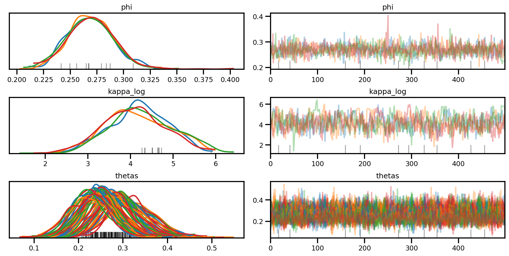
az.plot_trace(az_trace, compact=True);
az.plot_forest(az_trace,
               var_names=['thetas'],
               kind='ridgeplot',
               linewidth=4,
               combined=True,
               ridgeplot_overlap=1.5,
               figsize=(9, 8));
מודל אפקט מעורב (ראדון)
המודל האחרון doc PyMC3: פריימר על שיטות בייס עבור דוגמנות מדורגת
כמה שינויים בקודם (קנה מידה קטן יותר וכו')
טען נתונים גולמיים ונקה
srrs2 = pd.read_csv('https://raw.githubusercontent.com/pymc-devs/pymc3/master/pymc3/examples/data/srrs2.dat')

srrs2.columns = srrs2.columns.map(str.strip)
srrs_mn = srrs2[srrs2.state=='MN'].copy()
srrs_mn['fips'] = srrs_mn.stfips*1000 + srrs_mn.cntyfips

cty = pd.read_csv('https://raw.githubusercontent.com/pymc-devs/pymc3/master/pymc3/examples/data/cty.dat')
cty_mn = cty[cty.st=='MN'].copy()
cty_mn[ 'fips'] = 1000*cty_mn.stfips + cty_mn.ctfips

srrs_mn = srrs_mn.merge(cty_mn[['fips', 'Uppm']], on='fips')
srrs_mn = srrs_mn.drop_duplicates(subset='idnum')
u = np.log(srrs_mn.Uppm)

n = len(srrs_mn)

srrs_mn.county = srrs_mn.county.map(str.strip)
mn_counties = srrs_mn.county.unique()
counties = len(mn_counties)
county_lookup = dict(zip(mn_counties, range(len(mn_counties))))

county = srrs_mn['county_code'] = srrs_mn.county.replace(county_lookup).values
radon = srrs_mn.activity
srrs_mn['log_radon'] = log_radon = np.log(radon + 0.1).values
floor_measure = srrs_mn.floor.values.astype('float')

# Create new variable for mean of floor across counties
xbar = srrs_mn.groupby('county')['floor'].mean().rename(county_lookup).values
עבור מודלים עם טרנספורמציה מורכבת, יישום זה בסגנון פונקציונלי יקל על הכתיבה והבדיקה הרבה יותר. כמו כן, זה מקל בהרבה על יצירת פונקציית log_prob המותנית על (מיני-אצווה) של נתונים מוזנים באופן תכנותי:
def affine(u_val, x_county, county, floor, gamma, eps, b):
  """Linear equation of the coefficients and the covariates, with broadcasting."""
  return (tf.transpose((gamma[..., 0]
                      + gamma[..., 1]*u_val[:, None]
                      + gamma[..., 2]*x_county[:, None]))
          + tf.gather(eps, county, axis=-1)
          + b*floor)


def gen_radon_model(u_val, x_county, county, floor,
                    mu0=tf.zeros([], dtype, name='mu0')):
  """Creates a joint distribution representing our generative process."""
  return tfd.JointDistributionSequential([
      # sigma_a
      tfd.HalfCauchy(loc=mu0, scale=5.),
      # eps
      lambda sigma_a: tfd.Sample(
          tfd.Normal(loc=mu0, scale=sigma_a), sample_shape=counties),
      # gamma
      tfd.Sample(tfd.Normal(loc=mu0, scale=100.), sample_shape=3),
      # b
      tfd.Sample(tfd.Normal(loc=mu0, scale=100.), sample_shape=1),
      # sigma_y
      tfd.Sample(tfd.HalfCauchy(loc=mu0, scale=5.), sample_shape=1),
      # likelihood
      lambda sigma_y, b, gamma, eps: tfd.Independent(
          tfd.Normal(
              loc=affine(u_val, x_county, county, floor, gamma, eps, b),
              scale=sigma_y
          ),
          reinterpreted_batch_ndims=1
      ),
  ])

contextual_effect2 = gen_radon_model(
    u.values,  xbar[county], county, floor_measure)

@tf.function(autograph=False)
def unnormalized_posterior_log_prob(sigma_a, gamma, eps, b, sigma_y):
  """Computes `joint_log_prob` pinned at `log_radon`."""
  return contextual_effect2.log_prob(
      [sigma_a, gamma, eps, b, sigma_y, log_radon])

assert [4] == unnormalized_posterior_log_prob(
    *contextual_effect2.sample(4)[:-1]).shape
samples = contextual_effect2.sample(4)
pprint([s.shape for s in samples])
[TensorShape([4]),
 TensorShape([4, 85]),
 TensorShape([4, 3]),
 TensorShape([4, 1]),
 TensorShape([4, 1]),
 TensorShape([4, 919])]
contextual_effect2.log_prob_parts(list(samples)[:-1] + [log_radon])
[<tf.Tensor: shape=(4,), dtype=float64, numpy=array([-3.95681828, -2.45693443, -2.53310078, -4.7717536 ])>,
 <tf.Tensor: shape=(4,), dtype=float64, numpy=array([-340.65975204, -217.11139018, -246.50498667, -369.79687704])>,
 <tf.Tensor: shape=(4,), dtype=float64, numpy=array([-20.49822449, -20.38052557, -18.63843525, -17.83096972])>,
 <tf.Tensor: shape=(4,), dtype=float64, numpy=array([-5.94765605, -5.91460848, -6.66169402, -5.53894593])>,
 <tf.Tensor: shape=(4,), dtype=float64, numpy=array([-2.10293999, -4.34186631, -2.10744955, -3.016717  ])>,
 <tf.Tensor: shape=(4,), dtype=float64, numpy=
 array([-29022322.1413861 ,   -114422.36893361,  -8708500.81752865,
           -35061.92497235])>]
הסקה וריאציונית
תכונה מאוד חזקה אחד JointDistribution* היא שאתה יכול ליצור קירוב בקלות שישית. לדוגמה, כדי לעשות את meanfield ADVI, אתה פשוט בודק את הגרף ומחליף את כל ההתפלגות שלא נצפתה בהתפלגות נורמלית.
Meanfield ADVI
אתה יכול גם להשתמש בתכונת experimential ב tensorflow_probability / Python / ניסיוני / vi לבנות קירוב וריאציה, אשר הם בעצם אותו ההיגיון בשימוש מתחת (כלומר, באמצעות JointDistribution כדי קירוב לבנות), אבל עם תפוקת הקירוב במרחב המקורי במקום שטח בלתי מוגבל.
from tensorflow_probability.python.mcmc.transformed_kernel import (
    make_transform_fn, make_transformed_log_prob)
# Wrap logp so that all parameters are in the Real domain
# copied and edited from tensorflow_probability/python/mcmc/transformed_kernel.py
unconstraining_bijectors = [
    tfb.Exp(),
    tfb.Identity(),
    tfb.Identity(),
    tfb.Identity(),
    tfb.Exp()
]

unnormalized_log_prob = lambda *x: contextual_effect2.log_prob(x + (log_radon,))

contextual_effect_posterior = make_transformed_log_prob(
    unnormalized_log_prob,
    unconstraining_bijectors,
    direction='forward',
    # TODO(b/72831017): Disable caching until gradient linkage
    # generally works.
    enable_bijector_caching=False)
# debug
if True:
  # Check the two versions of log_prob - they should be different given the Jacobian
  rv_samples = contextual_effect2.sample(4)

  _inverse_transform = make_transform_fn(unconstraining_bijectors, 'inverse')
  _forward_transform = make_transform_fn(unconstraining_bijectors, 'forward')

  pprint([
      unnormalized_log_prob(*rv_samples[:-1]),
      contextual_effect_posterior(*_inverse_transform(rv_samples[:-1])),
      unnormalized_log_prob(
          *_forward_transform(
              tf.zeros_like(a, dtype=dtype) for a in rv_samples[:-1])
      ),
      contextual_effect_posterior(
          *[tf.zeros_like(a, dtype=dtype) for a in rv_samples[:-1]]
      ),
  ])
[<tf.Tensor: shape=(4,), dtype=float64, numpy=array([-1.73354969e+04, -5.51622488e+04, -2.77754609e+08, -1.09065161e+07])>,
 <tf.Tensor: shape=(4,), dtype=float64, numpy=array([-1.73331358e+04, -5.51582029e+04, -2.77754602e+08, -1.09065134e+07])>,
 <tf.Tensor: shape=(4,), dtype=float64, numpy=array([-1992.10420767, -1992.10420767, -1992.10420767, -1992.10420767])>,
 <tf.Tensor: shape=(4,), dtype=float64, numpy=array([-1992.10420767, -1992.10420767, -1992.10420767, -1992.10420767])>]
# Build meanfield ADVI for a jointdistribution
# Inspect the input jointdistribution and replace the list of distribution with
# a list of Normal distribution, each with the same shape.
def build_meanfield_advi(jd_list, observed_node=-1):
  """
  The inputted jointdistribution needs to be a batch version
  """
  # Sample to get a list of Tensors
  list_of_values = jd_list.sample(1)  # <== sample([]) might not work

  # Remove the observed node
  list_of_values.pop(observed_node)

  # Iterate the list of Tensor to a build a list of Normal distribution (i.e.,
  # the Variational posterior)
  distlist = []
  for i, value in enumerate(list_of_values):
    dtype = value.dtype
    rv_shape = value[0].shape
    loc = tf.Variable(
        tf.random.normal(rv_shape, dtype=dtype),
        name='meanfield_%s_mu' % i,
        dtype=dtype)
    scale = tfp.util.TransformedVariable(
        tf.fill(rv_shape, value=tf.constant(0.02, dtype)),
        tfb.Softplus(),
        name='meanfield_%s_scale' % i,
    )

    approx_node = tfd.Normal(loc=loc, scale=scale)
    if loc.shape == ():
      distlist.append(approx_node)
    else:
      distlist.append(
          # TODO: make the reinterpreted_batch_ndims more flexible (for
          # minibatch etc)
          tfd.Independent(approx_node, reinterpreted_batch_ndims=1)
      )

  # pass list to JointDistribution to initiate the meanfield advi
  meanfield_advi = tfd.JointDistributionSequential(distlist)
  return meanfield_advi
advi = build_meanfield_advi(contextual_effect2, observed_node=-1)

# Check the logp and logq
advi_samples = advi.sample(4)
pprint([
  advi.log_prob(advi_samples),
  contextual_effect_posterior(*advi_samples)
  ])
[<tf.Tensor: shape=(4,), dtype=float64, numpy=array([231.26836839, 229.40755095, 227.10287879, 224.05914594])>,
 <tf.Tensor: shape=(4,), dtype=float64, numpy=array([-10615.93542431, -11743.21420129, -10376.26732337, -11338.00600103])>]
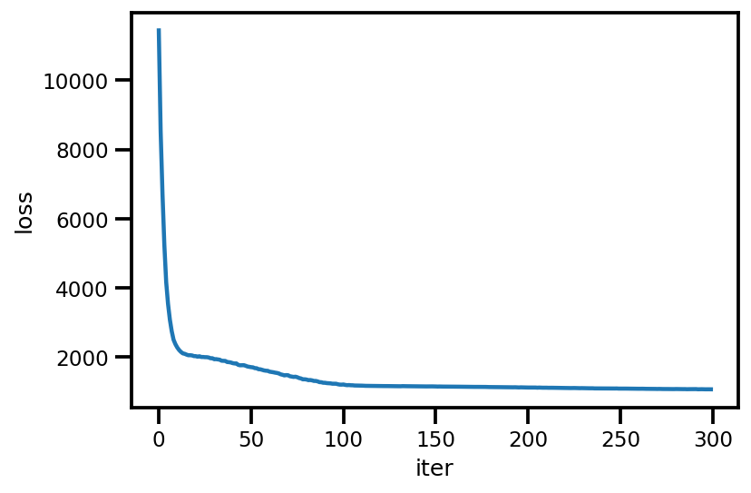
opt = tf.optimizers.Adam(learning_rate=.1)
@tf.function(experimental_compile=True)
def run_approximation():
loss_ = tfp.vi.fit_surrogate_posterior(
contextual_effect_posterior,
surrogate_posterior=advi,
optimizer=opt,
sample_size=10,
num_steps=300)
return loss_
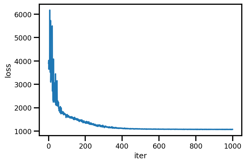
loss_ = run_approximation()
plt.plot(loss_);
plt.xlabel('iter');
plt.ylabel('loss');
graph_info = contextual_effect2.resolve_graph()
approx_param = dict()
free_param = advi.trainable_variables
for i, (rvname, param) in enumerate(graph_info[:-1]):
  approx_param[rvname] = {"mu": free_param[i*2].numpy(),
                          "sd": free_param[i*2+1].numpy()}
approx_param.keys()
dict_keys(['sigma_a', 'eps', 'gamma', 'b', 'sigma_y'])
approx_param['gamma']
{'mu': array([1.28145814, 0.70365287, 1.02689857]),
 'sd': array([-3.6604972 , -2.68153218, -2.04176524])}
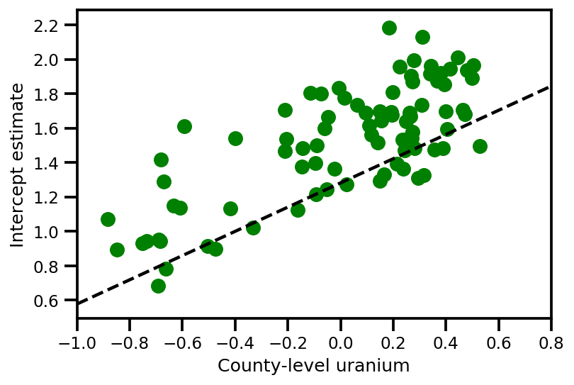
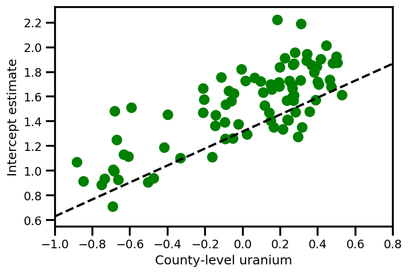
a_means = (approx_param['gamma']['mu'][0]
         + approx_param['gamma']['mu'][1]*u.values
         + approx_param['gamma']['mu'][2]*xbar[county]
         + approx_param['eps']['mu'][county])
_, index = np.unique(county, return_index=True)
plt.scatter(u.values[index], a_means[index], color='g')

xvals = np.linspace(-1, 0.8)
plt.plot(xvals,
         approx_param['gamma']['mu'][0]+approx_param['gamma']['mu'][1]*xvals,
         'k--')
plt.xlim(-1, 0.8)

plt.xlabel('County-level uranium');
plt.ylabel('Intercept estimate');
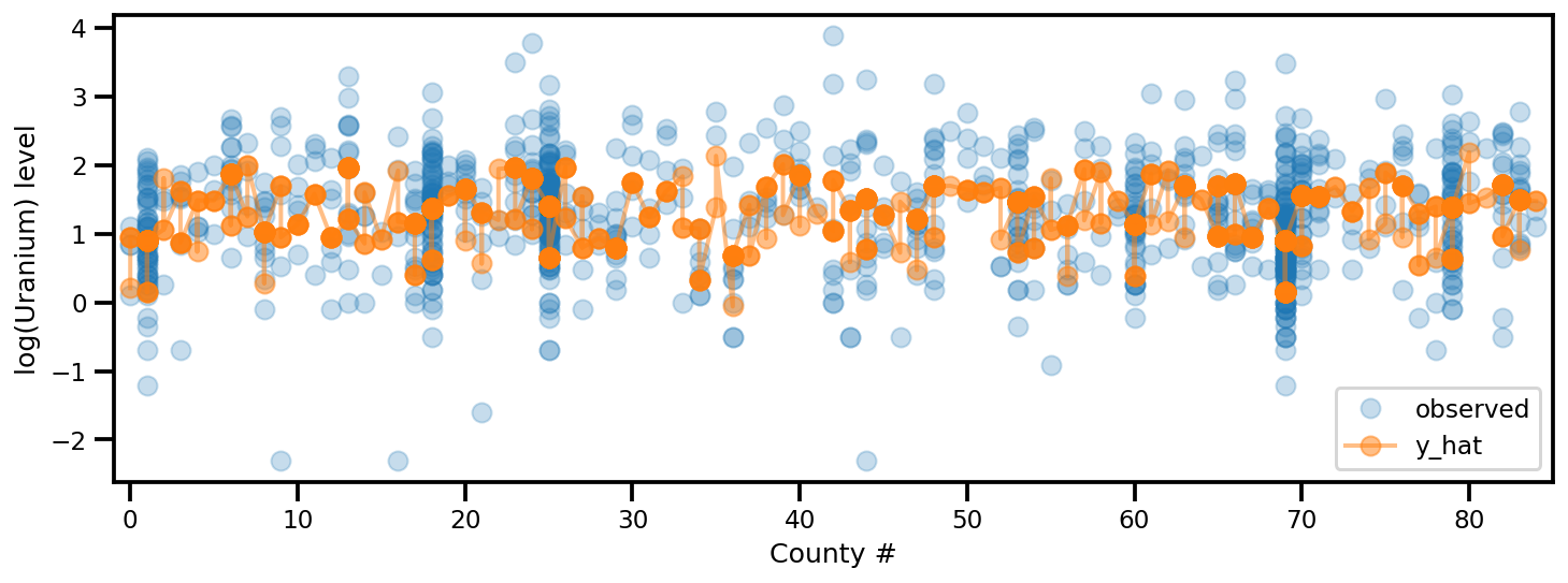
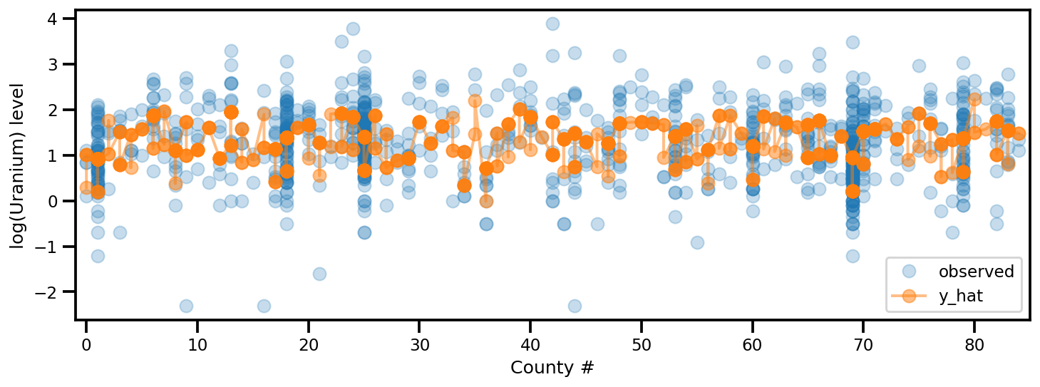
y_est = (approx_param['gamma']['mu'][0]
        + approx_param['gamma']['mu'][1]*u.values
        + approx_param['gamma']['mu'][2]*xbar[county]
        + approx_param['eps']['mu'][county]
        + approx_param['b']['mu']*floor_measure)

_, ax = plt.subplots(1, 1, figsize=(12, 4))
ax.plot(county, log_radon, 'o', alpha=.25, label='observed')
ax.plot(county, y_est, '-o', lw=2, alpha=.5, label='y_hat')
ax.set_xlim(-1, county.max()+1)
plt.legend(loc='lower right')
ax.set_xlabel('County #')
ax.set_ylabel('log(Uranium) level');
FullRank ADVI
לקבלת דרגה מלאה של ADVI, אנו רוצים להעריך את האחורי עם גאוס רב משתנים.
USE_FULLRANK = True
*prior_tensors, _ = contextual_effect2.sample()

mapper = Mapper(prior_tensors,
                [tfb.Identity() for _ in prior_tensors],
                contextual_effect2.event_shape[:-1])
rv_shape = ps.shape(mapper.flatten_and_concat(mapper.list_of_tensors))
init_val = tf.random.normal(rv_shape, dtype=dtype)
loc = tf.Variable(init_val, name='loc', dtype=dtype)

if USE_FULLRANK:
  # cov_param = tfp.util.TransformedVariable(
  #     10. * tf.eye(rv_shape[0], dtype=dtype),
  #     tfb.FillScaleTriL(),
  #     name='cov_param'
  #     )
  FillScaleTriL = tfb.FillScaleTriL(
        diag_bijector=tfb.Chain([
          tfb.Shift(tf.cast(.01, dtype)),
          tfb.Softplus(),
          tfb.Shift(tf.cast(np.log(np.expm1(1.)), dtype))]),
        diag_shift=None)
  cov_param = tfp.util.TransformedVariable(
      .02 * tf.eye(rv_shape[0], dtype=dtype),
      FillScaleTriL,
      name='cov_param')
  advi_approx = tfd.MultivariateNormalTriL(
      loc=loc, scale_tril=cov_param)
else:
  # An alternative way to build meanfield ADVI.
  cov_param = tfp.util.TransformedVariable(
      .02 * tf.ones(rv_shape, dtype=dtype),
      tfb.Softplus(),
      name='cov_param'
      )
  advi_approx = tfd.MultivariateNormalDiag(
      loc=loc, scale_diag=cov_param)

contextual_effect_posterior2 = lambda x: contextual_effect_posterior(
    *mapper.split_and_reshape(x)
)

# Check the logp and logq
advi_samples = advi_approx.sample(7)
pprint([
  advi_approx.log_prob(advi_samples),
  contextual_effect_posterior2(advi_samples)
  ])
[<tf.Tensor: shape=(7,), dtype=float64, numpy=
array([238.81841799, 217.71022639, 234.57207103, 230.0643819 ,
       243.73140943, 226.80149702, 232.85184209])>,
 <tf.Tensor: shape=(7,), dtype=float64, numpy=
array([-3638.93663169, -3664.25879314, -3577.69371677, -3696.25705312,
       -3689.12130489, -3777.53698383, -3659.4982734 ])>]
learning_rate = tf.optimizers.schedules.ExponentialDecay(
    initial_learning_rate=1e-2,
    decay_steps=10,
    decay_rate=0.99,
    staircase=True)

opt = tf.optimizers.Adam(learning_rate=learning_rate)

@tf.function(experimental_compile=True)
def run_approximation():
  loss_ = tfp.vi.fit_surrogate_posterior(
        contextual_effect_posterior2,
        surrogate_posterior=advi_approx,
        optimizer=opt,
        sample_size=10,
        num_steps=1000)
  return loss_

loss_ = run_approximation()
plt.plot(loss_);
plt.xlabel('iter');
plt.ylabel('loss');
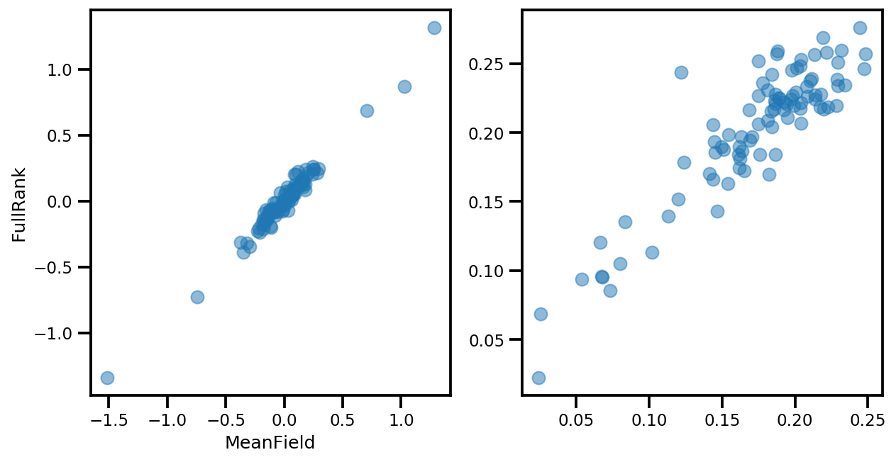
# debug
if True:
  _, ax = plt.subplots(1, 2, figsize=(10, 5))
  ax[0].plot(mapper.flatten_and_concat(advi.mean()), advi_approx.mean(), 'o', alpha=.5)
  ax[1].plot(mapper.flatten_and_concat(advi.stddev()), advi_approx.stddev(), 'o', alpha=.5)
  ax[0].set_xlabel('MeanField')
  ax[0].set_ylabel('FullRank')
graph_info = contextual_effect2.resolve_graph()
approx_param = dict()

free_param_mean = mapper.split_and_reshape(advi_approx.mean())
free_param_std = mapper.split_and_reshape(advi_approx.stddev())
for i, (rvname, param) in enumerate(graph_info[:-1]):
  approx_param[rvname] = {"mu": free_param_mean[i].numpy(),
                          "cov_info": free_param_std[i].numpy()}
a_means = (approx_param['gamma']['mu'][0]
         + approx_param['gamma']['mu'][1]*u.values
         + approx_param['gamma']['mu'][2]*xbar[county]
         + approx_param['eps']['mu'][county])
_, index = np.unique(county, return_index=True)
plt.scatter(u.values[index], a_means[index], color='g')

xvals = np.linspace(-1, 0.8)
plt.plot(xvals,
         approx_param['gamma']['mu'][0]+approx_param['gamma']['mu'][1]*xvals,
         'k--')
plt.xlim(-1, 0.8)

plt.xlabel('County-level uranium');
plt.ylabel('Intercept estimate');
y_est = (approx_param['gamma']['mu'][0]
         + approx_param['gamma']['mu'][1]*u.values
         + approx_param['gamma']['mu'][2]*xbar[county]
         + approx_param['eps']['mu'][county]
         + approx_param['b']['mu']*floor_measure)

_, ax = plt.subplots(1, 1, figsize=(12, 4))
ax.plot(county, log_radon, 'o', alpha=.25, label='observed')
ax.plot(county, y_est, '-o', lw=2, alpha=.5, label='y_hat')
ax.set_xlim(-1, county.max()+1)
plt.legend(loc='lower right')
ax.set_xlabel('County #')
ax.set_ylabel('log(Uranium) level');
דגם תערובת בטא-ברנולי
מודל תערובת שבו מבקרים רבים מסמנים פריטים מסוימים, עם תוויות סמויות לא ידועות (אמיתיות).
dtype = tf.float32
n = 50000    # number of examples reviewed
p_bad_ = 0.1 # fraction of bad events
m = 5        # number of reviewers for each example
rcl_ = .35 + np.random.rand(m)/10
prc_ = .65 + np.random.rand(m)/10

# PARAMETER TRANSFORMATION
tpr = rcl_
fpr = p_bad_*tpr*(1./prc_-1.)/(1.-p_bad_)
tnr = 1 - fpr

# broadcast to m reviewer.
batch_prob = np.asarray([tpr, fpr]).T
mixture = tfd.Mixture(
    tfd.Categorical(
        probs=[p_bad_, 1-p_bad_]),
    [
        tfd.Independent(tfd.Bernoulli(probs=tpr), 1),
        tfd.Independent(tfd.Bernoulli(probs=fpr), 1),
    ])
# Generate reviewer response
X_tf = mixture.sample([n])

# run once to always use the same array as input
# so we can compare the estimation from different
# inference method.
X_np = X_tf.numpy()
# batched Mixture model
mdl_mixture = tfd.JointDistributionSequential([
    tfd.Sample(tfd.Beta(5., 2.), m),
    tfd.Sample(tfd.Beta(2., 2.), m),
    tfd.Sample(tfd.Beta(1., 10), 1),
    lambda p_bad, rcl, prc: tfd.Sample(
        tfd.Mixture(
            tfd.Categorical(
                probs=tf.concat([p_bad, 1.-p_bad], -1)),
            [
              tfd.Independent(tfd.Bernoulli(
                  probs=rcl), 1),
              tfd.Independent(tfd.Bernoulli(
                  probs=p_bad*rcl*(1./prc-1.)/(1.-p_bad)), 1)
             ]
      ), (n, )),
    ])

mdl_mixture.resolve_graph()
(('prc', ()), ('rcl', ()), ('p_bad', ()), ('x', ('p_bad', 'rcl', 'prc')))
prc, rcl, p_bad, x = mdl_mixture.sample(4)
x.shape
TensorShape([4, 50000, 5])
mdl_mixture.log_prob_parts([prc, rcl, p_bad, X_np[np.newaxis, ...]])
[<tf.Tensor: shape=(4,), dtype=float32, numpy=array([1.4828572, 2.957961 , 2.9355168, 2.6116824], dtype=float32)>,
 <tf.Tensor: shape=(4,), dtype=float32, numpy=array([-0.14646745,  1.3308513 ,  1.1205603 ,  0.5441705 ], dtype=float32)>,
 <tf.Tensor: shape=(4,), dtype=float32, numpy=array([1.3733709, 1.8020535, 2.1865845, 1.5701319], dtype=float32)>,
 <tf.Tensor: shape=(4,), dtype=float32, numpy=array([-54326.664, -52683.93 , -64407.67 , -55007.895], dtype=float32)>]
מסקנות (NUTS)
nchain = 10
prc, rcl, p_bad, _ = mdl_mixture.sample(nchain)
initial_chain_state = [prc, rcl, p_bad]

# Since MCMC operates over unconstrained space, we need to transform the
# samples so they live in real-space.
unconstraining_bijectors = [
    tfb.Sigmoid(),       # Maps R to [0, 1].
    tfb.Sigmoid(),       # Maps R to [0, 1].
    tfb.Sigmoid(),       # Maps R to [0, 1].
]
step_size = [tf.cast(i, dtype=dtype) for i in [1e-3, 1e-3, 1e-3]]

X_expanded = X_np[np.newaxis, ...]
target_log_prob_fn = lambda *x: mdl_mixture.log_prob(x + (X_expanded, ))

samples, sampler_stat = run_chain(
    initial_chain_state, step_size, target_log_prob_fn,
    unconstraining_bijectors, burnin=100)
# using the pymc3 naming convention
sample_stats_name = ['lp', 'tree_size', 'diverging', 'energy', 'mean_tree_accept']
sample_stats = {k:v.numpy().T for k, v in zip(sample_stats_name, sampler_stat)}
sample_stats['tree_size'] = np.diff(sample_stats['tree_size'], axis=1)
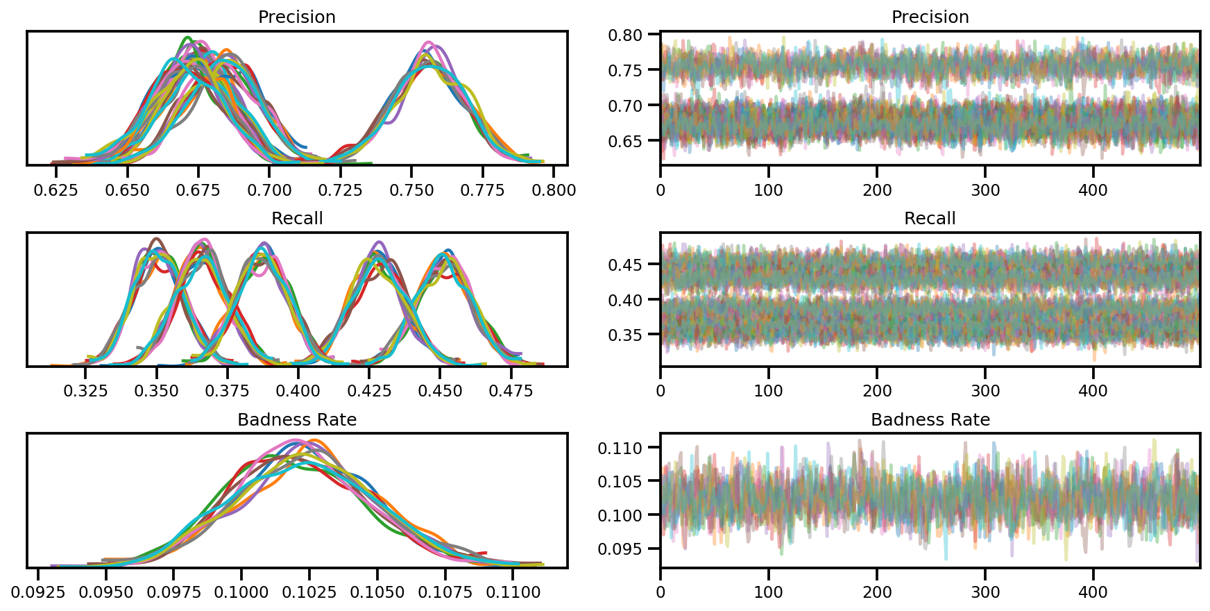
var_name = ['Precision', 'Recall', 'Badness Rate']
posterior = {k:np.swapaxes(v.numpy(), 1, 0)
for k, v in zip(var_name, samples)}
az_trace = az.from_dict(posterior=posterior, sample_stats=sample_stats)
axes = az.plot_trace(az_trace, compact=True);