
L'intento di questo notebook è quello di aiutare TFP 0.12.1 a "prendere vita" tramite alcuni piccoli frammenti - piccole demo di cose che puoi ottenere con TFP.
| | |  Visualizza la fonte su GitHub Visualizza la fonte su GitHub | |
Installa e importa
!pip3 install -qU tensorflow==2.4.0 tensorflow_probability==0.12.1 tensorflow-datasets inference_gym

import tensorflow as tf
import tensorflow_probability as tfp
assert '0.12' in tfp.__version__, tfp.__version__
assert '2.4' in tf.__version__, tf.__version__

physical_devices = tf.config.list_physical_devices('CPU')
tf.config.set_logical_device_configuration(
    physical_devices[0],
    [tf.config.LogicalDeviceConfiguration(),
     tf.config.LogicalDeviceConfiguration()])

tfd = tfp.distributions
tfb = tfp.bijectors
tfpk = tfp.math.psd_kernels

import matplotlib.pyplot as plt
import numpy as np
import scipy.interpolate
import IPython
import seaborn as sns
from inference_gym import using_tensorflow as gym
import logging
Biiettori
Glow
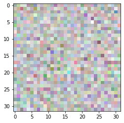
Un bijector dalla carta Glow: Flusso generativa con invertibile 1x1 Convoluzioni , da Kingma e Dhariwal.
Ecco come disegnare un'immagine da una distribuzione (nota che la distribuzione non ha "imparato" nulla qui).
image_shape = (32, 32, 4)  # 32 x 32 RGBA image

glow = tfb.Glow(output_shape=image_shape,
                coupling_bijector_fn=tfb.GlowDefaultNetwork,
                exit_bijector_fn=tfb.GlowDefaultExitNetwork)

pz = tfd.Sample(tfd.Normal(0., 1.), tf.reduce_prod(image_shape))

# Calling glow on distribution p(z) creates our glow distribution over images.
px = glow(pz)

# Take samples from the distribution to get images from your dataset.
image = px.sample(1)[0].numpy()

# Rescale to [0, 1].
image = (image - image.min()) / (image.max() - image.min())
plt.imshow(image);
RayleighCDF
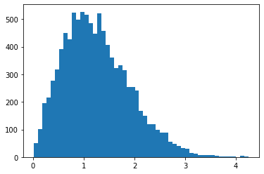
Bijector per la di distribuzione di Rayleigh CDF. Un uso è il campionamento dalla distribuzione di Rayleigh, prelevando campioni uniformi, quindi facendoli passare attraverso l'inverso del CDF.
bij = tfb.RayleighCDF()
uniforms = tfd.Uniform().sample(10_000)
plt.hist(bij.inverse(uniforms), bins='auto');
Ascending() sostituisce Invert(Ordered())
x = tfd.Normal(0., 1.).sample(5)
print(tfb.Ascending()(x))
print(tfb.Invert(tfb.Ordered())(x))
tf.Tensor([1.9363368 2.650928  3.4936204 4.1817293 5.6920815], shape=(5,), dtype=float32)
WARNING:tensorflow:From <ipython-input-5-1406b9939c00>:3: Ordered.__init__ (from tensorflow_probability.python.bijectors.ordered) is deprecated and will be removed after 2021-01-09.
Instructions for updating:
`Ordered` bijector is deprecated; please use `tfb.Invert(tfb.Ascending())` instead.
tf.Tensor([1.9363368 2.650928  3.4936204 4.1817293 5.6920815], shape=(5,), dtype=float32)
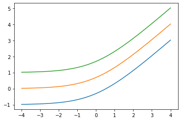
Aggiungere low arg: Softplus(low=2.)
x = tf.linspace(-4., 4., 100)

for low in (-1., 0., 1.):
  bij = tfb.Softplus(low=low)
  plt.plot(x, bij(x));
tfb.ScaleMatvecLinearOperatorBlock supporta blocco per blocco LinearOperator , args più parti
op_1 = tf.linalg.LinearOperatorDiag(diag=[1., -1., 3.])
op_2 = tf.linalg.LinearOperatorFullMatrix([[12., 5.], [-1., 3.]])
scale = tf.linalg.LinearOperatorBlockDiag([op_1, op_2], is_non_singular=True)

bij = tfb.ScaleMatvecLinearOperatorBlock(scale)
bij([[1., 2., 3.], [0., 1.]])
WARNING:tensorflow:From /usr/local/lib/python3.6/dist-packages/tensorflow/python/ops/linalg/linear_operator_block_diag.py:223: LinearOperator.graph_parents (from tensorflow.python.ops.linalg.linear_operator) is deprecated and will be removed in a future version.
Instructions for updating:
Do not call `graph_parents`.
[<tf.Tensor: shape=(3,), dtype=float32, numpy=array([ 1., -2.,  9.], dtype=float32)>,
 <tf.Tensor: shape=(2,), dtype=float32, numpy=array([5., 3.], dtype=float32)>]
distribuzioni
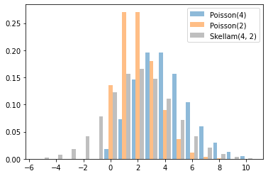
Skellam
Distribuzione sulle differenze di due Poisson camper. Si noti che i campioni di questa distribuzione possono essere negativi.
x = tf.linspace(-5., 10., 10 - -5 + 1)

rates = (4, 2)
for i, rate in enumerate(rates):
  plt.bar(x - .3 * (1 - i), tfd.Poisson(rate).prob(x), label=f'Poisson({rate})', alpha=0.5, width=.3)
plt.bar(x.numpy() + .3, tfd.Skellam(*rates).prob(x).numpy(), color='k', alpha=0.25, width=.3,
        label=f'Skellam{rates}')

plt.legend();
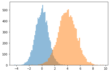
JointDistributionCoroutine[AutoBatched] prodotti namedtuple -come campioni
Specificare esplicitamente sample_dtype=[...] per il vecchio tuple comportamento.
@tfd.JointDistributionCoroutineAutoBatched
def model():
  x = yield tfd.Normal(0., 1., name='x')
  y = x + 4.
  yield tfd.Normal(y, 1., name='y')

draw = model.sample(10_000)

plt.hist(draw.x, bins='auto', alpha=0.5)
plt.hist(draw.y, bins='auto', alpha=0.5);
WARNING:tensorflow:Note that RandomStandardNormal inside pfor op may not give same output as inside a sequential loop.
WARNING:tensorflow:Note that RandomStandardNormal inside pfor op may not give same output as inside a sequential loop.
VonMisesFisher supporti dim > 5 , entropy()
La distribuzione di von Mises-Fisher è una distribuzione sul \(n-1\) dimensionale sfera in \(\mathbb{R}^n\).
dist = tfd.VonMisesFisher([0., 1, 0, 1, 0, 1], concentration=1.)
draws = dist.sample(3)

print(dist.entropy())
tf.reduce_sum(draws ** 2, axis=1)  # each draw has length 1
tf.Tensor(3.3533673, shape=(), dtype=float32)
<tf.Tensor: shape=(3,), dtype=float32, numpy=array([1.0000002 , 0.99999994, 1.0000001 ], dtype=float32)>
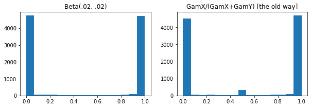
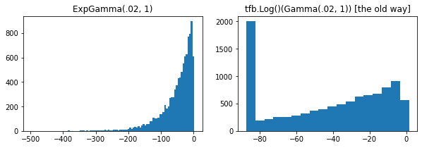
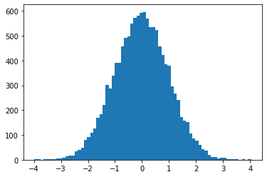
ExpGamma , ExpInverseGamma
log_rate parametro aggiunto alla Gamma . Miglioramenti numerici Quando si prelevano campioni a bassa concentrazione Beta , Dirichlet e amici. Gradienti di riparametrizzazione impliciti in tutti i casi.
plt.figure(figsize=(10, 3))
plt.subplot(121)
plt.hist(tfd.Beta(.02, .02).sample(10_000), bins='auto')
plt.title('Beta(.02, .02)')
plt.subplot(122)
plt.title('GamX/(GamX+GamY) [the old way]')
g = tfd.Gamma(.02, 1); s0, s1 = g.sample(10_000), g.sample(10_000)
plt.hist(s0 / (s0 + s1), bins='auto')
plt.show()

plt.figure(figsize=(10, 3))
plt.subplot(121)
plt.hist(tfd.ExpGamma(.02, 1.).sample(10_000), bins='auto')
plt.title('ExpGamma(.02, 1)')
plt.subplot(122)
plt.hist(tfb.Log()(tfd.Gamma(.02, 1.)).sample(10_000), bins='auto')
plt.title('tfb.Log()(Gamma(.02, 1)) [the old way]');
JointDistribution*AutoBatched supporta il campionamento riproducibili (con la lunghezza-2 tuple / semi Tensor)
@tfd.JointDistributionCoroutineAutoBatched
def model():
  x = yield tfd.Normal(0, 1, name='x')
  y = yield tfd.Normal(x + 4, 1, name='y')

print(model.sample(seed=(1, 2)))
print(model.sample(seed=(1, 2)))
StructTuple(
  x=<tf.Tensor: shape=(), dtype=float32, numpy=-0.59835213>,
  y=<tf.Tensor: shape=(), dtype=float32, numpy=6.2380724>
)
StructTuple(
  x=<tf.Tensor: shape=(), dtype=float32, numpy=-0.59835213>,
  y=<tf.Tensor: shape=(), dtype=float32, numpy=6.2380724>
)
KL(VonMisesFisher || SphericalUniform)
# Build vMFs with the same mean direction, batch of increasing concentrations.
vmf = tfd.VonMisesFisher(tf.math.l2_normalize(tf.random.normal([10])),
                         concentration=[0., .1, 1., 10.])
# KL increases with concentration, since vMF(conc=0) == SphericalUniform.
print(tfd.kl_divergence(vmf, tfd.SphericalUniform(10)))
tf.Tensor([4.7683716e-07 4.9877167e-04 4.9384594e-02 2.4844694e+00], shape=(4,), dtype=float32)
parameter_properties
Classi distribuzione ora esporre una parameter_properties(dtype=tf.float32, num_classes=None) Metodo di classe, che può consentire la costruzione automatica di numerose classi di distribuzioni.
print('Gamma:', tfd.Gamma.parameter_properties())
print('Categorical:', tfd.Categorical.parameter_properties(dtype=tf.float64, num_classes=7))
Gamma: {'concentration': ParameterProperties(event_ndims=0, shape_fn=<function ParameterProperties.<lambda> at 0x7ff6bbfcdd90>, default_constraining_bijector_fn=<function Gamma._parameter_properties.<locals>.<lambda> at 0x7ff6afd95510>, is_preferred=True), 'rate': ParameterProperties(event_ndims=0, shape_fn=<function ParameterProperties.<lambda> at 0x7ff6bbfcdd90>, default_constraining_bijector_fn=<function Gamma._parameter_properties.<locals>.<lambda> at 0x7ff6afd95ea0>, is_preferred=False), 'log_rate': ParameterProperties(event_ndims=0, shape_fn=<function ParameterProperties.<lambda> at 0x7ff6bbfcdd90>, default_constraining_bijector_fn=<class 'tensorflow_probability.python.bijectors.identity.Identity'>, is_preferred=True)}
Categorical: {'logits': ParameterProperties(event_ndims=1, shape_fn=<function Categorical._parameter_properties.<locals>.<lambda> at 0x7ff6afd95510>, default_constraining_bijector_fn=<class 'tensorflow_probability.python.bijectors.identity.Identity'>, is_preferred=True), 'probs': ParameterProperties(event_ndims=1, shape_fn=<function Categorical._parameter_properties.<locals>.<lambda> at 0x7ff6afdc91e0>, default_constraining_bijector_fn=<class 'tensorflow_probability.python.bijectors.softmax_centered.SoftmaxCentered'>, is_preferred=False)}
experimental_default_event_space_bijector
Ora accetta argomenti aggiuntivi che bloccano alcune parti di distribuzione.
@tfd.JointDistributionCoroutineAutoBatched
def model():
  scale = yield tfd.Gamma(1, 1, name='scale')
  obs = yield tfd.Normal(0, scale, name='obs')

model.experimental_default_event_space_bijector(obs=.2).forward(
    [tf.random.uniform([3], -2, 2.)])
StructTuple(
  scale=<tf.Tensor: shape=(3,), dtype=float32, numpy=array([0.6630705, 1.5401832, 1.0777743], dtype=float32)>
)
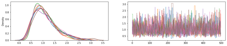
JointDistribution.experimental_pin
Perni alcune parti congiunte distribuzione corrispondente JointDistributionPinned oggetto che rappresenta la densità normalizzato giunto.
Lavorare con experimental_default_event_space_bijector , questo rende facendo inferenza variazionale o MCMC con default sensibili molto più semplice. Nel seguito esempio, le prime due righe del sample make esecuzione MCMC una brezza.
dist = tfd.JointDistributionSequential([
    tfd.HalfNormal(1.),
    lambda scale: tfd.Normal(0., scale, name='observed')])

@tf.function
def sample():
  bij = dist.experimental_default_event_space_bijector(observed=1.)
  target_log_prob = dist.experimental_pin(observed=1.).unnormalized_log_prob

  kernel = tfp.mcmc.TransformedTransitionKernel(
      tfp.mcmc.HamiltonianMonteCarlo(target_log_prob,
                                     step_size=0.6,
                                     num_leapfrog_steps=16),
      bijector=bij)
  return tfp.mcmc.sample_chain(500,
                               current_state=tf.ones([8]),  # multiple chains
                               kernel=kernel,
                               trace_fn=None)

draws = sample()

fig, (hist, trace) = plt.subplots(ncols=2, figsize=(16, 3))
trace.plot(draws, alpha=0.5)
for col in tf.transpose(draws):
  sns.kdeplot(col, ax=hist);
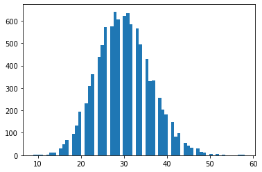
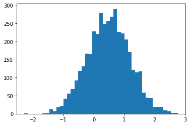
tfd.NegativeBinomial.experimental_from_mean_dispersion
Parametrizzazione alternativa. Invia un'e-mail a tfprobability@tensorflow.org o inviaci un PR per aggiungere metodi di classe simili per altre distribuzioni.
nb = tfd.NegativeBinomial.experimental_from_mean_dispersion(30., .01)
plt.hist(nb.sample(10_000), bins='auto');
tfp.experimental.distribute
DistributionStrategy -consapevoli distribuzioni congiunte, consentendo cross-device calcoli verosimiglianza. Sharded Independent e Sample distribuzioni.
# Note: 2-logical devices are configured in the install/import cell at top.
strategy = tf.distribute.MirroredStrategy()
assert strategy.num_replicas_in_sync == 2

@tfp.experimental.distribute.JointDistributionCoroutine
def model():
  root = tfp.experimental.distribute.JointDistributionCoroutine.Root
  group_scale = yield root(tfd.Sample(tfd.Exponential(1), 3, name='group_scale'))
  _ = yield tfp.experimental.distribute.ShardedSample(tfd.Independent(tfd.Normal(0, group_scale), 1),
                                                      sample_shape=[4], name='x')

seed1, seed2 = tfp.random.split_seed((1, 2))

@tf.function
def sample(seed):
  return model.sample(seed=seed)
xs = strategy.run(sample, (seed1,))
print("""
Note that the global latent `group_scale` is shared across devices, whereas
the local `x` is sampled independently on each device.
""")
print('sample:', xs)
print('another sample:', strategy.run(sample, (seed2,)))

@tf.function
def log_prob(x):
  return model.log_prob(x)
print("""
Note that each device observes the same log_prob (local latent log_probs are
summed across devices).
""")
print('log_prob:', strategy.run(log_prob, (xs,)))

@tf.function
def grad_log_prob(x):
  return tfp.math.value_and_gradient(model.log_prob, x)[1]

print("""
Note that each device observes the same log_prob gradient (local latents have
independent gradients, global latents have gradients aggregated across devices).
""")
print('grad_log_prob:', strategy.run(grad_log_prob, (xs,)))
WARNING:tensorflow:There are non-GPU devices in `tf.distribute.Strategy`, not using nccl allreduce.
INFO:tensorflow:Using MirroredStrategy with devices ('/job:localhost/replica:0/task:0/device:CPU:0', '/job:localhost/replica:0/task:0/device:CPU:1')

Note that the global latent `group_scale` is shared across devices, whereas
the local `x` is sampled independently on each device.

sample: StructTuple(
  group_scale=PerReplica:{
      0: <tf.Tensor: shape=(3,), dtype=float32, numpy=array([2.6355493, 1.1805456, 1.245112 ], dtype=float32)>,
      1: <tf.Tensor: shape=(3,), dtype=float32, numpy=array([2.6355493, 1.1805456, 1.245112 ], dtype=float32)>
    },
  x=PerReplica:{
      0: <tf.Tensor: shape=(2, 3), dtype=float32, numpy=
    array([[-0.90548456,  0.7675636 ,  0.27627748],
           [-0.3475989 ,  2.0194046 , -1.2531326 ]], dtype=float32)>,
      1: <tf.Tensor: shape=(2, 3), dtype=float32, numpy=
    array([[ 3.251305  , -0.5790973 ,  0.42745453],
           [-1.562331  ,  0.3006323 ,  0.635732  ]], dtype=float32)>
    }
)
another sample: StructTuple(
  group_scale=PerReplica:{
      0: <tf.Tensor: shape=(3,), dtype=float32, numpy=array([2.41133   , 0.10307606, 0.5236566 ], dtype=float32)>,
      1: <tf.Tensor: shape=(3,), dtype=float32, numpy=array([2.41133   , 0.10307606, 0.5236566 ], dtype=float32)>
    },
  x=PerReplica:{
      0: <tf.Tensor: shape=(2, 3), dtype=float32, numpy=
    array([[-3.2476294 ,  0.07213175, -0.39536062],
           [-1.2319602 , -0.05505352,  0.06356457]], dtype=float32)>,
      1: <tf.Tensor: shape=(2, 3), dtype=float32, numpy=
    array([[ 5.6028705 ,  0.11919801, -0.48446828],
           [-1.5938259 ,  0.21123725,  0.28979057]], dtype=float32)>
    }
)

Note that each device observes the same log_prob (local latent log_probs are
summed across devices).

INFO:tensorflow:Reduce to /job:localhost/replica:0/task:0/device:CPU:0 then broadcast to ('/job:localhost/replica:0/task:0/device:CPU:0', '/job:localhost/replica:0/task:0/device:CPU:1').
log_prob: PerReplica:{
  0: tf.Tensor(-25.05747, shape=(), dtype=float32),
  1: tf.Tensor(-25.05747, shape=(), dtype=float32)
}

Note that each device observes the same log_prob gradient (local latents have
independent gradients, global latents are aggregated across devices).

INFO:tensorflow:Reduce to /job:localhost/replica:0/task:0/device:CPU:0 then broadcast to ('/job:localhost/replica:0/task:0/device:CPU:0', '/job:localhost/replica:0/task:0/device:CPU:1').
INFO:tensorflow:Reduce to /job:localhost/replica:0/task:0/device:CPU:0 then broadcast to ('/job:localhost/replica:0/task:0/device:CPU:0', '/job:localhost/replica:0/task:0/device:CPU:1').
grad_log_prob: StructTuple(
  group_scale=PerReplica:{
      0: <tf.Tensor: shape=(3,), dtype=float32, numpy=array([-1.7555585, -1.2928739, -3.0554674], dtype=float32)>,
      1: <tf.Tensor: shape=(3,), dtype=float32, numpy=array([-1.7555585, -1.2928739, -3.0554674], dtype=float32)>
    },
  x=PerReplica:{
      0: <tf.Tensor: shape=(2, 3), dtype=float32, numpy=
    array([[ 0.13035832, -0.5507428 , -0.17820862],
           [ 0.05004217, -1.4489648 ,  0.80831426]], dtype=float32)>,
      1: <tf.Tensor: shape=(2, 3), dtype=float32, numpy=
    array([[-0.46807498,  0.41551432, -0.27572307],
           [ 0.22492138, -0.21570992, -0.41006932]], dtype=float32)>
    }
)
Kernel PSD
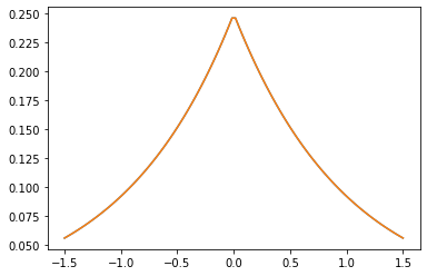
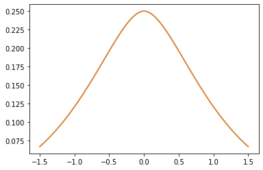
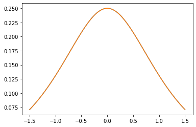
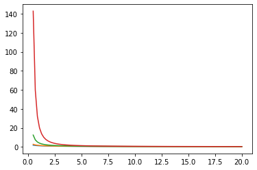
GeneralizedMatern
Il GeneralizedMatern positiva semidefinita kernel generalizza MaternOneHalf , MAterhThreeHalves e MaternFiveHalves .
gm = tfpk.GeneralizedMatern(df=[0.5, 1.5, 2.5], length_scale=1., amplitude=0.5)
m1 = tfpk.MaternOneHalf(length_scale=1., amplitude=0.5)
m2 = tfpk.MaternThreeHalves(length_scale=1., amplitude=0.5)
m3 = tfpk.MaternFiveHalves(length_scale=1., amplitude=0.5)
xs = tf.linspace(-1.5, 1.5, 100)

gm_matrix = gm.matrix([[0.]], xs[..., tf.newaxis])
plt.plot(xs, gm_matrix[0][0])
plt.plot(xs, m1.matrix([[0.]], xs[..., tf.newaxis])[0])
plt.show()
plt.plot(xs, gm_matrix[1][0])
plt.plot(xs, m2.matrix([[0.]], xs[..., tf.newaxis])[0])
plt.show()
plt.plot(xs, gm_matrix[2][0])
plt.plot(xs, m3.matrix([[0.]], xs[..., tf.newaxis])[0])
plt.show()
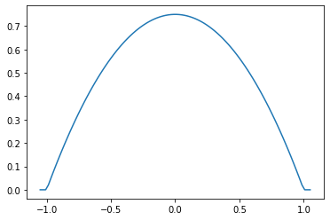
Parabolic (Epanechnikov)
epa = tfpk.Parabolic()
xs = tf.linspace(-1.05, 1.05, 100)
plt.plot(xs, epa.matrix([[0.]], xs[..., tf.newaxis])[0]);
VI
build_asvi_surrogate_posterior
Costruisci automaticamente un surrogato posteriore strutturato per VI in un modo che incorpori la struttura grafica della distribuzione precedente. Questo utilizza il metodo descritto nel documento automatico Structured Variazionali Inference ( https://arxiv.org/abs/2002.00643 ).
# Import a Brownian Motion model from TFP's inference gym.
model = gym.targets.BrownianMotionMissingMiddleObservations()
prior = model.prior_distribution()
ground_truth = ground_truth = model.sample_transformations['identity'].ground_truth_mean
target_log_prob = lambda *values: model.log_likelihood(values) + prior.log_prob(values)
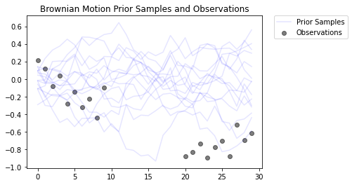
Questo modella un processo di moto browniano con un modello di osservazione gaussiano. Consiste di 30 timestep, ma i 10 timestep centrali non sono osservabili.
  locs[0] ~ Normal(loc=0, scale=innovation_noise_scale)
  for t in range(1, num_timesteps):
    locs[t] ~ Normal(loc=locs[t - 1], scale=innovation_noise_scale)

  for t in range(num_timesteps):
    observed_locs[t] ~ Normal(loc=locs[t], scale=observation_noise_scale)
L'obiettivo è quello di dedurre i valori delle locs da osservazioni rumorosi ( observed_locs ). Poiché al centro 10 Timesteps sono osservabili, observed_locs sono NaN valori a Timesteps [10,19].
# The observed loc values in the Brownian Motion inference gym model
OBSERVED_LOC = np.array([
    0.21592641, 0.118771404, -0.07945447, 0.037677474, -0.27885845, -0.1484156,
    -0.3250906, -0.22957903, -0.44110894, -0.09830782, np.nan, np.nan, np.nan,
    np.nan, np.nan, np.nan, np.nan, np.nan, np.nan, np.nan, -0.8786016,
    -0.83736074, -0.7384849, -0.8939254, -0.7774566, -0.70238715, -0.87771565,
    -0.51853573, -0.6948214, -0.6202789
]).astype(dtype=np.float32)

# Plot the prior and the likelihood observations
plt.figure()
plt.title('Brownian Motion Prior Samples and Observations')

num_samples = 15
prior_samples = prior.sample(num_samples)

plt.plot(prior_samples, c='blue', alpha=0.1)
plt.plot(prior_samples[0][0], label="Prior Samples", c='blue', alpha=0.1)

plt.scatter(x=range(30),y=OBSERVED_LOC, c='black', alpha=0.5, label="Observations")

plt.legend(bbox_to_anchor=(1.05, 1), borderaxespad=0.);
logging.getLogger('tensorflow').setLevel(logging.ERROR)  # suppress pfor warnings

# Construct and train an ASVI Surrogate Posterior.
asvi_surrogate_posterior = tfp.experimental.vi.build_asvi_surrogate_posterior(prior)

asvi_losses = tfp.vi.fit_surrogate_posterior(target_log_prob,
                                        asvi_surrogate_posterior,
                                        optimizer=tf.optimizers.Adam(learning_rate=0.1),
                                        num_steps=500)
logging.getLogger('tensorflow').setLevel(logging.NOTSET)
# Construct and train a Mean-Field Surrogate Posterior.
factored_surrogate_posterior = tfp.experimental.vi.build_factored_surrogate_posterior(event_shape=prior.event_shape)

factored_losses = tfp.vi.fit_surrogate_posterior(target_log_prob,
                                        factored_surrogate_posterior,
                                        optimizer=tf.optimizers.Adam(learning_rate=0.1),
                                        num_steps=500)
logging.getLogger('tensorflow').setLevel(logging.ERROR)  # suppress pfor warnings

# Sample from the posteriors.
asvi_posterior_samples = asvi_surrogate_posterior.sample(num_samples)
factored_posterior_samples = factored_surrogate_posterior.sample(num_samples)

logging.getLogger('tensorflow').setLevel(logging.NOTSET)
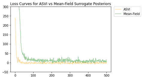
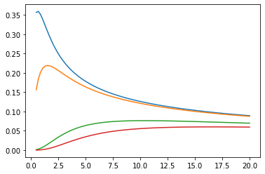
Sia l'ASVI che la distribuzione posteriore surrogata del campo medio sono convergenti e la distribuzione posteriore surrogata dell'ASVI ha avuto una perdita finale inferiore (valore ELBO negativo).
# Plot the loss curves.
plt.figure()
plt.title('Loss Curves for ASVI vs Mean-Field Surrogate Posteriors')

plt.plot(asvi_losses, c='orange', label='ASVI', alpha = 0.4)
plt.plot(factored_losses, c='green', label='Mean-Field', alpha = 0.4)
plt.ylim(-50, 300)

plt.legend(bbox_to_anchor=(1.3, 1), borderaxespad=0.);
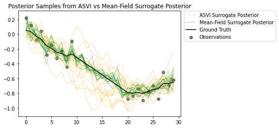
I campioni dei posteriori evidenziano quanto bene il surrogato posteriore ASVI catturi l'incertezza per i tempi senza osservazioni. D'altra parte, il surrogato posteriore del campo medio lotta per catturare la vera incertezza.
# Plot samples from the ASVI and Mean-Field Surrogate Posteriors.
plt.figure()
plt.title('Posterior Samples from ASVI vs Mean-Field Surrogate Posterior')

plt.plot(asvi_posterior_samples, c='orange', alpha = 0.25)
plt.plot(asvi_posterior_samples[0][0], label='ASVI Surrogate Posterior', c='orange', alpha = 0.25)

plt.plot(factored_posterior_samples, c='green', alpha = 0.25)
plt.plot(factored_posterior_samples[0][0], label='Mean-Field Surrogate Posterior', c='green', alpha = 0.25)

plt.scatter(x=range(30),y=OBSERVED_LOC, c='black', alpha=0.5, label='Observations')

plt.plot(ground_truth, c='black', label='Ground Truth')

plt.legend(bbox_to_anchor=(1.585, 1), borderaxespad=0.);
MCMC
ProgressBarReducer
Visualizza l'avanzamento del campionatore. (Potrebbe avere una riduzione delle prestazioni nominali; attualmente non supportato nella compilazione JIT.)
kernel = tfp.mcmc.HamiltonianMonteCarlo(lambda x: -x**2 / 2, .05, 20)
pbar = tfp.experimental.mcmc.ProgressBarReducer(100)
kernel = tfp.experimental.mcmc.WithReductions(kernel, pbar)
plt.hist(tf.reshape(tfp.mcmc.sample_chain(100, current_state=tf.ones([128]), kernel=kernel, trace_fn=None), [-1]), bins='auto')
pbar.bar.close()
99%|█████████▉| 99/100 [00:03<00:00, 27.37it/s]
sample_sequential_monte_carlo supporta il campionamento riproducibili
initial_state = tf.random.uniform([4096], -2., 2.)
def smc(seed):
  return tfp.experimental.mcmc.sample_sequential_monte_carlo(
    prior_log_prob_fn=lambda x: -x**2 / 2,
    likelihood_log_prob_fn=lambda x: -(x-1.)**2 / 2,
    current_state=initial_state,
    seed=seed)[1]
plt.hist(smc(seed=(12, 34)), bins='auto');plt.show()

print(smc(seed=(12, 34))[:10])
print('different:', smc(seed=(10, 20))[:10])
print('same:', smc(seed=(12, 34))[:10])
tf.Tensor(
[ 0.665834    0.9892149   0.7961128   1.0016634  -1.000767   -0.19461267
  1.3070581   1.127177    0.9940303   0.58239716], shape=(10,), dtype=float32)
different: tf.Tensor(
[ 1.3284367   0.4374407   1.1349089   0.4557473   0.06510283 -0.08954388
  1.1735026   0.8170528   0.12443061  0.34413314], shape=(10,), dtype=float32)
same: tf.Tensor(
[ 0.665834    0.9892149   0.7961128   1.0016634  -1.000767   -0.19461267
  1.3070581   1.127177    0.9940303   0.58239716], shape=(10,), dtype=float32)
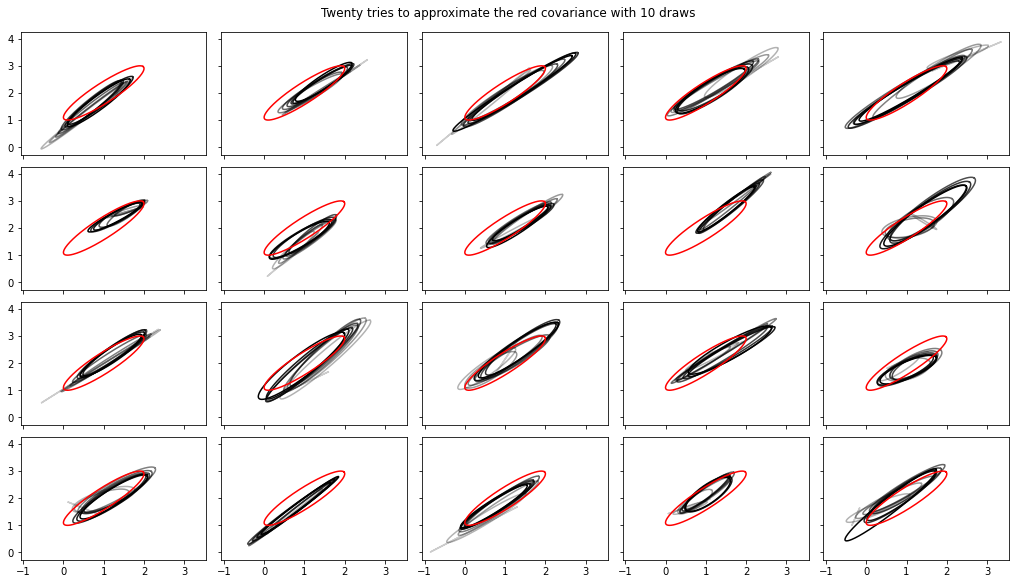
Aggiunti calcoli in streaming di varianza, covarianza, Rhat
Nota, le interfacce a queste sono cambiate un po 'in tfp-nightly .
def cov_to_ellipse(t, cov, mean):
  """Draw a one standard deviation ellipse from the mean, according to cov."""
  diag = tf.linalg.diag_part(cov)
  a = 0.5 * tf.reduce_sum(diag)
  b = tf.sqrt(0.25 * (diag[0] - diag[1])**2 + cov[0, 1]**2)
  major = a + b
  minor = a - b
  theta = tf.math.atan2(major - cov[0, 0], cov[0, 1])
  x = (tf.sqrt(major) * tf.cos(theta) * tf.cos(t) -
       tf.sqrt(minor) * tf.sin(theta) * tf.sin(t))
  y = (tf.sqrt(major) * tf.sin(theta) * tf.cos(t) +
       tf.sqrt(minor) * tf.cos(theta) * tf.sin(t))
  return x + mean[0], y + mean[1]

fig, axes = plt.subplots(nrows=4, ncols=5, figsize=(14, 8),
                         sharex=True, sharey=True, constrained_layout=True)
t = tf.linspace(0., 2 * np.pi, 200)
tot = 10
cov = 0.1 * tf.eye(2) + 0.9 * tf.ones([2, 2])
mvn = tfd.MultivariateNormalTriL(loc=[1., 2.],
                                 scale_tril=tf.linalg.cholesky(cov))

for ax in axes.ravel():
  rv = tfp.experimental.stats.RunningCovariance(
      num_samples=0., mean=tf.zeros(2), sum_squared_residuals=tf.zeros((2, 2)),
      event_ndims=1)

  for idx, x in enumerate(mvn.sample(tot)):
    rv = rv.update(x)
    ax.plot(*cov_to_ellipse(t, rv.covariance(), rv.mean),
            color='k', alpha=(idx + 1) / tot)
  ax.plot(*cov_to_ellipse(t, mvn.covariance(), mvn.mean()), 'r')
fig.suptitle("Twenty tries to approximate the red covariance with 10 draws");
Matematica, statistiche
Funzioni di Bessel: ive, kve, log-ive
xs = tf.linspace(0.5, 20., 100)
ys = tfp.math.bessel_ive([[0.5], [1.], [np.pi], [4.]], xs)
zs = tfp.math.bessel_kve([[0.5], [1.], [2.], [np.pi]], xs)

for i in range(4):
  plt.plot(xs, ys[i])
plt.show()

for i in range(4):
  plt.plot(xs, zs[i])
plt.show()
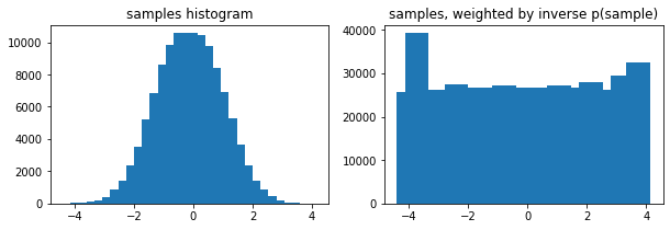
Opzionali weights arg a tfp.stats.histogram
edges = tf.linspace(-4., 4, 31)
samps = tfd.TruncatedNormal(0, 1, -4, 4).sample(100_000, seed=(123, 456))
_, (ax1, ax2) = plt.subplots(1, 2, figsize=(10, 3))
ax1.bar(edges[:-1], tfp.stats.histogram(samps, edges))
ax1.set_title('samples histogram')
ax2.bar(edges[:-1], tfp.stats.histogram(samps, edges, weights=1 / tfd.Normal(0, 1).prob(samps)))
ax2.set_title('samples, weighted by inverse p(sample)');
tfp.math.erfcinv
x = tf.linspace(-3., 3., 10)
y = tf.math.erfc(x)
z = tfp.math.erfcinv(y)
print(x)
print(z)
tf.Tensor(
[-3.         -2.3333333  -1.6666666  -1.         -0.33333325  0.3333335

  1.          1.666667    2.3333335   3.        ], shape=(10,), dtype=float32)
tf.Tensor(
[-3.0002644  -2.3333426  -1.6666666  -0.9999997  -0.3333332   0.33333346
  0.9999999   1.6666667   2.3333335   3.0000002 ], shape=(10,), dtype=float32)