TensorFlow powraca na Google I/O 14 maja! Zarejestruj się teraz

Ta strona została przetłumaczona przez Cloud Translation API.

Notatnik z informacjami o wersji TFP (0.13.0)

Zamiarem tego notebooka jest pomóc TFP 0.13.0 „ożyć” za pomocą kilku małych fragmentów – małych demonstracji rzeczy, które można osiągnąć za pomocą TFP.

Zobacz na TensorFlow.org

Uruchom w Google Colab

Wyświetl źródło na GitHub

Pobierz notatnik

Instalacje i importy

!pip3 install -qU tensorflow==2.5.0 tensorflow_probability==0.13.0 tensorflow-datasets inference_gym

import tensorflow as tf
import tensorflow_probability as tfp
assert '0.13' in tfp.__version__, tfp.__version__
assert '2.5' in tf.__version__, tf.__version__

physical_devices = tf.config.list_physical_devices('CPU')
tf.config.set_logical_device_configuration(
    physical_devices[0],
    [tf.config.LogicalDeviceConfiguration(),
     tf.config.LogicalDeviceConfiguration()])

tfd = tfp.distributions
tfb = tfp.bijectors
tfpk = tfp.math.psd_kernels

import matplotlib.pyplot as plt
import numpy as np
import scipy.interpolate
import IPython
import seaborn as sns
import logging

[K     |████████████████████████████████| 5.4MB 8.8MB/s 
[K     |████████████████████████████████| 3.9MB 37.1MB/s 
[K     |████████████████████████████████| 296kB 31.6MB/s 
[?25h

Dystrybucje [matematyka podstawowa]

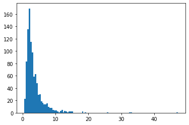
`BetaQuotient`

Stosunek dwóch niezależnych zmiennych losowych o rozkładzie beta

plt.hist(tfd.BetaQuotient(concentration1_numerator=5.,
                          concentration0_numerator=2.,
                          concentration1_denominator=3.,
                          concentration0_denominator=8.).sample(1_000, seed=(1, 23)),
         bins='auto');

png

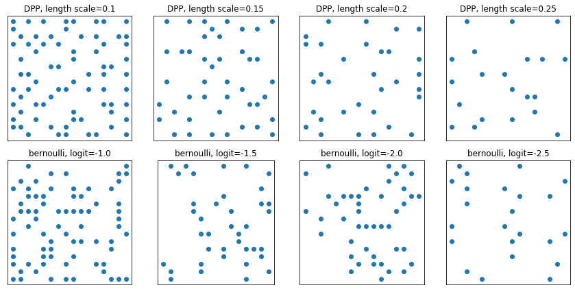
`DeterminantalPointProcess`

Rozkład na podzbiory (reprezentowane jako jeden gorący) danego zbioru. Próbki mają właściwość odpychania (prawdopodobieństwa są proporcjonalne do objętości rozpiętej przez wektory odpowiadające wybranemu podzbiorowi punktów), która ma tendencję do próbkowania różnych podzbiorów. [Porównaj z próbkami iid Bernoulliego.]

grid_size = 16
# Generate grid_size**2 pts on the unit square.
grid = np.arange(0, 1, 1./grid_size).astype(np.float32)
import itertools
points = np.array(list(itertools.product(grid, grid)))

# Create the kernel L that parameterizes the DPP.
kernel_amplitude = 2.
kernel_lengthscale = [.1, .15, .2, .25]  # Increasing length scale indicates more points are "nearby", tending toward smaller subsets.
kernel = tfpk.ExponentiatedQuadratic(kernel_amplitude, kernel_lengthscale)
kernel_matrix = kernel.matrix(points, points)

eigenvalues, eigenvectors = tf.linalg.eigh(kernel_matrix)
dpp = tfd.DeterminantalPointProcess(eigenvalues, eigenvectors)
print(dpp)

# The inner-most dimension of the result of `dpp.sample` is a multi-hot
# encoding of a subset of {1, ..., ground_set_size}.
# We will compare against a bernoulli distribution.
samps_dpp = dpp.sample(seed=(1, 2))  # 4 x grid_size**2
logits = tf.broadcast_to([[-1.], [-1.5], [-2], [-2.5]], [4, grid_size**2])
samps_bern = tfd.Bernoulli(logits=logits).sample(seed=(2, 3))

plt.figure(figsize=(12, 6))
for i, (samp, samp_bern) in enumerate(zip(samps_dpp, samps_bern)):
  plt.subplot(241 + i)
  plt.scatter(*points[np.where(samp)].T)
  plt.title(f'DPP, length scale={kernel_lengthscale[i]}')
  plt.xticks([])
  plt.yticks([])
  plt.gca().set_aspect(1.)
  plt.subplot(241 + i + 4)
  plt.scatter(*points[np.where(samp_bern)].T)
  plt.title(f'bernoulli, logit={logits[i,0]}')
  plt.xticks([])
  plt.yticks([])
  plt.gca().set_aspect(1.)

plt.tight_layout()
plt.show()

tfp.distributions.DeterminantalPointProcess("DeterminantalPointProcess", batch_shape=[4], event_shape=[256], dtype=int32)

png

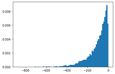
`SigmoidBeta`

Logarytmiczne szanse dwóch rozkładów gamma. Więcej numerycznie stabilny przestrzeń próbka niż Beta .

plt.hist(tfd.SigmoidBeta(concentration1=.01, concentration0=2.).sample(10_000, seed=(1, 23)),
         bins='auto', density=True);
plt.show()

print('Old way, fractions non-finite:')
print(np.sum(~tf.math.is_finite(
    tfb.Invert(tfb.Sigmoid())(tfd.Beta(concentration1=.01, concentration0=2.)).sample(10_000, seed=(1, 23)))) / 10_000)
print(np.sum(~tf.math.is_finite(
    tfb.Invert(tfb.Sigmoid())(tfd.Beta(concentration1=2., concentration0=.01)).sample(10_000, seed=(2, 34)))) / 10_000)

png

Old way, fractions non-finite:
0.4215
0.8624

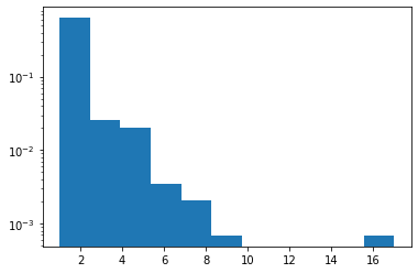
Zipf

Dodano obsługę JAX.

plt.hist(tfd.Zipf(3.).sample(1_000, seed=(12, 34)).numpy(), bins='auto', density=True, log=True);

png

`NormalInverseGaussian`

Elastyczna rodzina parametryczna obsługująca ciężkie ogony, skośne i waniliowe Normal.

`MatrixNormalLinearOperator`

Macierz Rozkład normalny.

# Initialize a single 2 x 3 Matrix Normal.
mu = [[1., 2, 3], [3., 4, 5]]
col_cov = [[ 0.36,  0.12,  0.06],
           [ 0.12,  0.29, -0.13],
           [ 0.06, -0.13,  0.26]]
scale_column = tf.linalg.LinearOperatorLowerTriangular(tf.linalg.cholesky(col_cov))
scale_row = tf.linalg.LinearOperatorDiag([0.9, 0.8])

mvn = tfd.MatrixNormalLinearOperator(loc=mu, scale_row=scale_row, scale_column=scale_column)
mvn.sample()

WARNING:tensorflow:From /usr/local/lib/python3.7/dist-packages/tensorflow/python/ops/linalg/linear_operator_kronecker.py:224: LinearOperator.graph_parents (from tensorflow.python.ops.linalg.linear_operator) is deprecated and will be removed in a future version.
Instructions for updating:
Do not call `graph_parents`.
<tf.Tensor: shape=(2, 3), dtype=float32, numpy=
array([[1.2495145, 1.549366 , 3.2748342],
       [3.7330258, 4.3413105, 4.83423  ]], dtype=float32)>

`MatrixStudentTLinearOperator`

Rozkład macierzy T.

mu = [[1., 2, 3], [3., 4, 5]]
col_cov = [[ 0.36,  0.12,  0.06],
           [ 0.12,  0.29, -0.13],
           [ 0.06, -0.13,  0.26]]
scale_column = tf.linalg.LinearOperatorLowerTriangular(tf.linalg.cholesky(col_cov))
scale_row = tf.linalg.LinearOperatorDiag([0.9, 0.8])

mvn = tfd.MatrixTLinearOperator(
    df=2.,
    loc=mu,
    scale_row=scale_row,
    scale_column=scale_column)
mvn.sample()

<tf.Tensor: shape=(2, 3), dtype=float32, numpy=
array([[1.6549466, 2.6708362, 2.8629923],
       [2.1222284, 3.6904747, 5.08014  ]], dtype=float32)>

Dystrybucje [oprogramowanie / wrappery]

`Sharded`

Odłamuje niezależne fragmenty zdarzeń dystrybucji na wiele procesorów. Kruszywa log_prob różnych urządzeniach, uchwyty gradienty w porozumieniu z tfp.experimental.distribute.JointDistribution* . Znacznie więcej w Ukazuje Inference notebooka.

strategy = tf.distribute.MirroredStrategy()

@tf.function
def sample_and_lp(seed):
  d = tfp.experimental.distribute.Sharded(tfd.Normal(0, 1))
  s = d.sample(seed=seed)
  return s, d.log_prob(s)

strategy.run(sample_and_lp, args=(tf.constant([12,34]),))

WARNING:tensorflow:There are non-GPU devices in `tf.distribute.Strategy`, not using nccl allreduce.
WARNING:tensorflow:Collective ops is not configured at program startup. Some performance features may not be enabled.
INFO:tensorflow:Using MirroredStrategy with devices ('/job:localhost/replica:0/task:0/device:CPU:0', '/job:localhost/replica:0/task:0/device:CPU:1')
INFO:tensorflow:Reduce to /job:localhost/replica:0/task:0/device:CPU:0 then broadcast to ('/job:localhost/replica:0/task:0/device:CPU:0', '/job:localhost/replica:0/task:0/device:CPU:1').
(PerReplica:{
   0: <tf.Tensor: shape=(), dtype=float32, numpy=0.0051413667>,
   1: <tf.Tensor: shape=(), dtype=float32, numpy=-0.3393052>
 }, PerReplica:{
   0: <tf.Tensor: shape=(), dtype=float32, numpy=-1.8954543>,
   1: <tf.Tensor: shape=(), dtype=float32, numpy=-1.8954543>
 })

`BatchBroadcast`

Niejawnie nadawanie wymiarów wsad dystrybucji bazowego z lub do danego kształtu wsadowym.

underlying = tfd.MultivariateNormalDiag(tf.zeros([7, 1, 5]), tf.ones([5]))
print('underlying:', underlying)

d = tfd.BatchBroadcast(underlying, [8, 1, 6])
print('broadcast [7, 1] *with* [8, 1, 6]:', d)

try:
  tfd.BatchBroadcast(underlying, to_shape=[8, 1, 6])
except ValueError as e:
  print('broadcast [7, 1] *to* [8, 1, 6] is invalid:', e)

d = tfd.BatchBroadcast(underlying, to_shape=[8, 7, 6])
print('broadcast [7, 1] *to* [8, 7, 6]:', d)

underlying: tfp.distributions.MultivariateNormalDiag("MultivariateNormalDiag", batch_shape=[7, 1], event_shape=[5], dtype=float32)
broadcast [7, 1] *with* [8, 1, 6]: tfp.distributions.BatchBroadcast("BatchBroadcastMultivariateNormalDiag", batch_shape=[8, 7, 6], event_shape=[5], dtype=float32)
broadcast [7, 1] *to* [8, 1, 6] is invalid: Argument `to_shape` ([8 1 6]) is incompatible with underlying distribution batch shape ((7, 1)).
broadcast [7, 1] *to* [8, 7, 6]: tfp.distributions.BatchBroadcast("BatchBroadcastMultivariateNormalDiag", batch_shape=[8, 7, 6], event_shape=[5], dtype=float32)

`Masked`

Dla pojedynczego programu / wielu danych jednostkowych lub rozrzedzony-as-zamaskowanych gęsty użytkowych przypadkach, dystrybucji, maski na zewnątrz log_prob nieprawidłowych wypłat bazowych.

d = tfd.Masked(tfd.Normal(tf.zeros([7]), 1), 
               validity_mask=tf.sequence_mask([3, 4], 7))
print(d.log_prob(d.sample(seed=(1, 1))))

d = tfd.Masked(tfd.Normal(0, 1), 
               validity_mask=[False, True, False],
               safe_sample_fn=tfd.Distribution.mode)
print(d.log_prob(d.sample(seed=(2, 2))))

tf.Tensor(
[[-2.3054113 -1.8524303 -1.2220721  0.         0.         0.

   0.       ]
 [-1.118623  -1.1370811 -1.1574132 -5.884986   0.         0.
   0.       ]], shape=(2, 7), dtype=float32)
tf.Tensor([ 0.         -0.93683904  0.        ], shape=(3,), dtype=float32)

Bijektory

Bijektory
- Dodaj bijectors naśladować tf.nest.flatten ( tfb.tree_flatten ) i tf.nest.pack_sequence_as ( tfb.pack_sequence_as ).
- Dodaje tfp.experimental.bijectors.Sharded
- Usunąć przestarzałe tfb.ScaleTrilL . Zastosowanie tfb.FillScaleTriL zamiast.
- Dodaje cls.parameter_properties() adnotacje dotyczące Bijectors.
- Rozszerzyć zakres tfb.Power dla wszystkich liczb rzeczywistych dla nieparzystych potęg całkowitych.
- Wywnioskuj log-deg-jacobian bijektorów skalarnych przy użyciu autodiff, jeśli nie określono inaczej.

Restrukturyzacyjne bijektory

ex = (tf.constant(1.), dict(b=tf.constant(2.), c=tf.constant(3.)))
b = tfb.tree_flatten(ex)
print(b.forward(ex))
print(b.inverse(list(tf.constant([1., 2, 3]))))

b = tfb.pack_sequence_as(ex)
print(b.forward(list(tf.constant([1., 2, 3]))))
print(b.inverse(ex))

[<tf.Tensor: shape=(), dtype=float32, numpy=1.0>, <tf.Tensor: shape=(), dtype=float32, numpy=2.0>, <tf.Tensor: shape=(), dtype=float32, numpy=3.0>]
(<tf.Tensor: shape=(), dtype=float32, numpy=1.0>, {'b': <tf.Tensor: shape=(), dtype=float32, numpy=2.0>, 'c': <tf.Tensor: shape=(), dtype=float32, numpy=3.0>})
(<tf.Tensor: shape=(), dtype=float32, numpy=1.0>, {'b': <tf.Tensor: shape=(), dtype=float32, numpy=2.0>, 'c': <tf.Tensor: shape=(), dtype=float32, numpy=3.0>})
[<tf.Tensor: shape=(), dtype=float32, numpy=1.0>, <tf.Tensor: shape=(), dtype=float32, numpy=2.0>, <tf.Tensor: shape=(), dtype=float32, numpy=3.0>]

`Sharded`

Redukcja SPMD w wyznaczniku logarytmicznym. Zobacz Sharded w rozkładzie poniżej.

strategy = tf.distribute.MirroredStrategy()

def sample_lp_logdet(seed):
  d = tfd.TransformedDistribution(tfp.experimental.distribute.Sharded(tfd.Normal(0, 1), shard_axis_name='i'),
                                  tfp.experimental.bijectors.Sharded(tfb.Sigmoid(), shard_axis_name='i'))
  s = d.sample(seed=seed)
  return s, d.log_prob(s), d.bijector.inverse_log_det_jacobian(s)
strategy.run(sample_lp_logdet, (tf.constant([1, 2]),))

WARNING:tensorflow:There are non-GPU devices in `tf.distribute.Strategy`, not using nccl allreduce.
WARNING:tensorflow:Collective ops is not configured at program startup. Some performance features may not be enabled.
INFO:tensorflow:Using MirroredStrategy with devices ('/job:localhost/replica:0/task:0/device:CPU:0', '/job:localhost/replica:0/task:0/device:CPU:1')
WARNING:tensorflow:Using MirroredStrategy eagerly has significant overhead currently. We will be working on improving this in the future, but for now please wrap `call_for_each_replica` or `experimental_run` or `run` inside a tf.function to get the best performance.
INFO:tensorflow:Reduce to /job:localhost/replica:0/task:0/device:CPU:0 then broadcast to ('/job:localhost/replica:0/task:0/device:CPU:0', '/job:localhost/replica:0/task:0/device:CPU:1').
INFO:tensorflow:Reduce to /job:localhost/replica:0/task:0/device:CPU:0 then broadcast to ('/job:localhost/replica:0/task:0/device:CPU:0', '/job:localhost/replica:0/task:0/device:CPU:1').
(PerReplica:{
   0: <tf.Tensor: shape=(), dtype=float32, numpy=0.87746525>,
   1: <tf.Tensor: shape=(), dtype=float32, numpy=0.24580425>
 }, PerReplica:{
   0: <tf.Tensor: shape=(), dtype=float32, numpy=-0.48870325>,
   1: <tf.Tensor: shape=(), dtype=float32, numpy=-0.48870325>
 }, PerReplica:{
   0: <tf.Tensor: shape=(), dtype=float32, numpy=3.9154015>,
   1: <tf.Tensor: shape=(), dtype=float32, numpy=3.9154015>
 })

VI

Dodaje build_split_flow_surrogate_posterior do tfp.experimental.vi zbudować strukturę VI zastępczych tyłki z przepływów normalizujące.
Dodaje build_affine_surrogate_posterior do tfp.experimental.vi na budowę ADVI posteriors zastępczych z kształtu zdarzeń.
Dodaje build_affine_surrogate_posterior_from_base_distribution do tfp.experimental.vi aby umożliwić budowę posteriors ADVI zastępczych ze strukturami korelacji indukowanych przez transformacje afiniczne.

VI/MAP/MLE

Dodano metoda wygoda tfp.experimental.util.make_trainable(cls) , aby utworzyć wyszkolić wystąpień dystrybucji i bijectors.

d = tfp.experimental.util.make_trainable(tfd.Gamma)
print(d.trainable_variables)
print(d)

(<tf.Variable 'Gamma_trainable_variables/concentration:0' shape=() dtype=float32, numpy=1.0296053>, <tf.Variable 'Gamma_trainable_variables/log_rate:0' shape=() dtype=float32, numpy=-0.3465951>)
tfp.distributions.Gamma("Gamma", batch_shape=[], event_shape=[], dtype=float32)

MCMC

Diagnostyka MCMC obsługuje dowolne struktury stanów, a nie tylko listy.
remc_thermodynamic_integrals dodano do tfp.experimental.mcmc
Dodaje tfp.experimental.mcmc.windowed_adaptive_hmc
Dodaje eksperymentalny interfejs API do inicjowania łańcucha Markowa z niemal zerowej jednolitej dystrybucji w nieograniczonej przestrzeni. tfp.experimental.mcmc.init_near_unconstrained_zero
Dodaje eksperymentalne narzędzie do ponawiania próby inicjalizacji łańcucha Markowa do momentu znalezienia akceptowalnego punktu. tfp.experimental.mcmc.retry_init
Tasowanie eksperymentalnego interfejsu API MCMC do przesyłania strumieniowego w celu umieszczenia go w tfp.mcmc z minimalnymi zakłóceniami.
Dodaje ThinningKernel do experimental.mcmc .
Dodaje experimental.mcmc.run_kernel kierowca jako kandydata strumieniowe oparte na zastępstwo mcmc.sample_chain

`init_near_unconstrained_zero` , `retry_init`

@tfd.JointDistributionCoroutine
def model():
  Root = tfd.JointDistributionCoroutine.Root
  c0 = yield Root(tfd.Gamma(2, 2, name='c0'))
  c1 = yield Root(tfd.Gamma(2, 2, name='c1'))
  counts = yield tfd.Sample(tfd.BetaBinomial(23, c1, c0), 10, name='counts')
jd = model.experimental_pin(counts=model.sample(seed=[20, 30]).counts)

init_dist = tfp.experimental.mcmc.init_near_unconstrained_zero(jd)
print(init_dist)

tfp.experimental.mcmc.retry_init(init_dist.sample, jd.unnormalized_log_prob)

tfp.distributions.TransformedDistribution("default_joint_bijectorrestructureJointDistributionSequential", batch_shape=StructTuple(
  c0=[],
  c1=[]
), event_shape=StructTuple(
  c0=[],
  c1=[]
), dtype=StructTuple(
  c0=float32,
  c1=float32
))
StructTuple(
  c0=<tf.Tensor: shape=(), dtype=float32, numpy=1.7879653>,
  c1=<tf.Tensor: shape=(), dtype=float32, numpy=0.34548905>
)

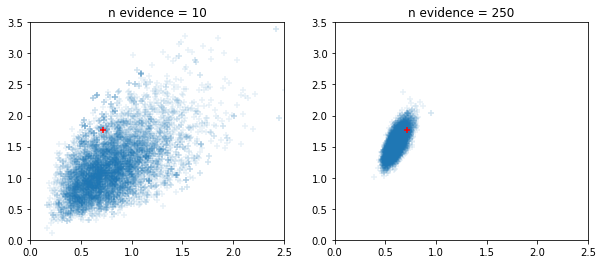
Okienkowe adaptacyjne próbniki HMC i NUTS

fig, ax = plt.subplots(1, 2, figsize=(10, 4))
for i, n_evidence in enumerate((10, 250)):
  ax[i].set_title(f'n evidence = {n_evidence}')
  ax[i].set_xlim(0, 2.5); ax[i].set_ylim(0, 3.5)
  @tfd.JointDistributionCoroutine
  def model():
    Root = tfd.JointDistributionCoroutine.Root
    c0 = yield Root(tfd.Gamma(2, 2, name='c0'))
    c1 = yield Root(tfd.Gamma(2, 2, name='c1'))
    counts = yield tfd.Sample(tfd.BetaBinomial(23, c1, c0), n_evidence, name='counts')
  s = model.sample(seed=[20, 30])
  print(s)
  jd = model.experimental_pin(counts=s.counts)
  states, trace = tf.function(tfp.experimental.mcmc.windowed_adaptive_hmc)(
      100, jd, num_leapfrog_steps=5, seed=[100, 200])
  ax[i].scatter(states.c0.numpy().reshape(-1), states.c1.numpy().reshape(-1), 
                marker='+', alpha=.1)
  ax[i].scatter(s.c0, s.c1, marker='+', color='r')

StructTuple(
  c0=<tf.Tensor: shape=(), dtype=float32, numpy=0.7161876>,
  c1=<tf.Tensor: shape=(), dtype=float32, numpy=1.7696666>,
  counts=<tf.Tensor: shape=(10,), dtype=float32, numpy=array([ 6., 10., 23.,  7.,  2., 20., 14., 16., 22., 17.], dtype=float32)>
)
WARNING:tensorflow:6 out of the last 6 calls to <function windowed_adaptive_hmc at 0x7fda42bed8c0> triggered tf.function retracing. Tracing is expensive and the excessive number of tracings could be due to (1) creating @tf.function repeatedly in a loop, (2) passing tensors with different shapes, (3) passing Python objects instead of tensors. For (1), please define your @tf.function outside of the loop. For (2), @tf.function has experimental_relax_shapes=True option that relaxes argument shapes that can avoid unnecessary retracing. For (3), please refer to https://www.tensorflow.org/guide/function#controlling_retracing and https://www.tensorflow.org/api_docs/python/tf/function for  more details.
StructTuple(
  c0=<tf.Tensor: shape=(), dtype=float32, numpy=0.7161876>,
  c1=<tf.Tensor: shape=(), dtype=float32, numpy=1.7696666>,
  counts=<tf.Tensor: shape=(250,), dtype=float32, numpy=
    array([ 6., 10., 23.,  7.,  2., 20., 14., 16., 22., 17., 22., 21.,  6.,
           21., 12., 22., 23., 16., 18., 21., 16., 17., 17., 16., 21., 14.,
           23., 15., 10., 19.,  8., 23., 23., 14.,  1., 23., 16., 22., 20.,
           20., 22., 15., 16., 20., 20., 21., 23., 22., 21., 15., 18., 23.,
           12., 16., 19., 23., 18.,  5., 22., 22., 22., 18., 12., 17., 17.,
           16.,  8., 22., 20., 23.,  3., 12., 14., 18.,  7., 19., 19.,  9.,
           10., 23., 14., 22., 22., 21., 13., 23., 14., 23., 10., 17., 23.,
           17., 20., 16., 20., 19., 14.,  0., 17., 22., 12.,  2., 17., 15.,
           14., 23., 19., 15., 23.,  2., 21., 23., 21.,  7., 21., 12., 23.,
           17., 17.,  4., 22., 16., 14., 19., 19., 20.,  6., 16., 14., 18.,
           21., 12., 21., 21., 22.,  2., 19., 11.,  6., 19.,  1., 23., 23.,
           14.,  6., 23., 18.,  8., 20., 23., 13., 20., 18., 23., 17., 22.,
           23., 20., 18., 22., 16., 23.,  9., 22., 21., 16., 20., 21., 16.,
           23.,  7., 13., 23., 19.,  3., 13., 23., 23., 13., 19., 23., 20.,
           18.,  8., 19., 14., 12.,  6.,  8., 23.,  3., 13., 21., 23., 22.,
           23., 19., 22., 21., 15., 22., 21., 21., 23.,  9., 19., 20., 23.,
           11., 23., 14., 23., 14., 21., 21., 10., 23.,  9., 13.,  1.,  8.,
            8., 20., 21., 21., 21., 14., 16., 16.,  9., 23., 22., 11., 23.,
           12., 18.,  1., 23.,  9.,  3., 21., 21., 23., 22., 18., 23., 16.,
            3., 11., 16.], dtype=float32)>
)

png

Matematyka, statystyki

Matematyka/linalg
- Dodaj tfp.math.trapz o trapezoidalnym integracji.
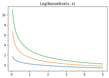
- Dodaj tfp.math.log_bessel_kve .
- Dodaj no_pivot_ldl do experimental.linalg .
- Dodaj marginal_fn argument GaussianProcess (patrz no_pivot_ldl ).
- Dodano tfp.math.atan_difference(x, y)
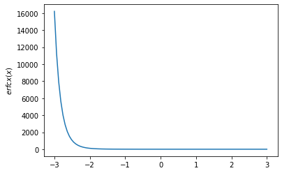
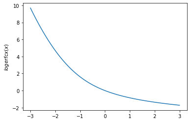
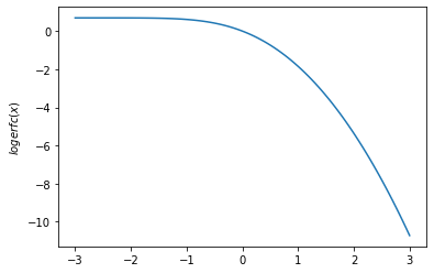
- Dodaj tfp.math.erfcx , tfp.math.logerfc i tfp.math.logerfcx
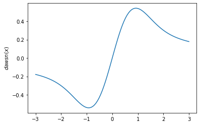
- Dodaj tfp.math.dawsn za integralną Dawsona.
- Dodaj tfp.math.igammaincinv , tfp.math.igammacinv .
- Dodaj tfp.math.sqrt1pm1 .
- Dodaj LogitNormal.stddev_approx i LogitNormal.variance_approx
- Dodaj tfp.math.owens_t do funkcji Owena T.
- Dodaj bracket_root metodę automatycznie zainicjować granicach do poszukiwania korzeni.
- Dodaj metodę Chandrupatli do znajdowania pierwiastków funkcji skalarnych.
Statystyki
- tfp.stats.windowed_mean sprawnie wylicza okienkowym środków.
- tfp.stats.windowed_variance sprawnie i dokładnie Oblicza okienkiem wariancje.
- tfp.stats.cumulative_variance wydajnie i precyzyjnie oblicza skumulowane wariancji.
- RunningCovariance i znajomi mogą teraz zostać zainicjowana z przykładu Tensor, nie tylko z wyraźnego kształtu i dtype.
- Cleaner API dla RunningCentralMoments , RunningMean , RunningPotentialScaleReduction .

Funkcje Owena T, Erfcx, Logerfc, Logerfcx, Dawson

# Owen's T gives the probability that X > h, 0 < Y < a * X. Let's check that
# with random sampling.
h = np.array([1., 2.]).astype(np.float32)
a = np.array([10., 11.5]).astype(np.float32)
probs = tfp.math.owens_t(h, a)

x = tfd.Normal(0., 1.).sample(int(1e5), seed=(6, 245)).numpy()
y = tfd.Normal(0., 1.).sample(int(1e5), seed=(7, 245)).numpy()

true_values = (
    (x[..., np.newaxis] > h) &
    (0. < y[..., np.newaxis]) &
    (y[..., np.newaxis] < a * x[..., np.newaxis]))

print('Calculated values: {}'.format(
    np.count_nonzero(true_values, axis=0) / 1e5))

print('Expected values: {}'.format(probs))

Calculated values: [0.07896 0.01134]
Expected values: [0.07932763 0.01137507]

x = np.linspace(-3., 3., 100)
plt.plot(x, tfp.math.erfcx(x))
plt.ylabel('$erfcx(x)$')
plt.show()

plt.plot(x, tfp.math.logerfcx(x))
plt.ylabel('$logerfcx(x)$')
plt.show()

plt.plot(x, tfp.math.logerfc(x))
plt.ylabel('$logerfc(x)$')
plt.show()

plt.plot(x, tfp.math.dawsn(x))
plt.ylabel('$dawsn(x)$')
plt.show()

png

igammainv / igammacinv

# Igammainv and Igammacinv are inverses to Igamma and Igammac

x = np.linspace(1., 10., 10)
y = tf.math.igamma(0.3, x)
x_prime = tfp.math.igammainv(0.3, y)
print('x: {}'.format(x))
print('igammainv(igamma(a, x)):\n {}'.format(x_prime))

y = tf.math.igammac(0.3, x)
x_prime = tfp.math.igammacinv(0.3, y)

print('\n')
print('x: {}'.format(x))
print('igammacinv(igammac(a, x)):\n {}'.format(x_prime))

x: [ 1.  2.  3.  4.  5.  6.  7.  8.  9. 10.]
igammainv(igamma(a, x)):
 [1.        1.9999992 3.000003  4.0000024 5.0000257 5.999887  7.0002484
 7.999243  8.99872   9.994673 ]


x: [ 1.  2.  3.  4.  5.  6.  7.  8.  9. 10.]
igammacinv(igammac(a, x)):
 [1.       2.       3.       4.       5.       6.       7.       8.000001

 9.       9.999999]

log-kve

x = np.linspace(0., 5., 100)
for v in [0.5, 2., 3]:
  plt.plot(x, tfp.math.log_bessel_kve(v, x).numpy())

plt.title('Log(BesselKve(v, x)')

Text(0.5, 1.0, 'Log(BesselKve(v, x)')

png

Inny

STS
- Przyspieszenie STS prognozowania i rozkładu przy użyciu wewnętrznego tf.function opakowania.
- Dodaj opcję, aby przyspieszyć filtrowania w LinearGaussianSSM gdy wymagane są wyniki tylko Ostatnim krokiem jest.
- Wariacyjna Wnioskowanie ze wspólnych rozkładów: przykład notebook z modelem Radon .
- Dodaj eksperymentalne wsparcie dla przekształcenia dowolnej dystrybucji w bijektora wstępnego kondycjonowania.
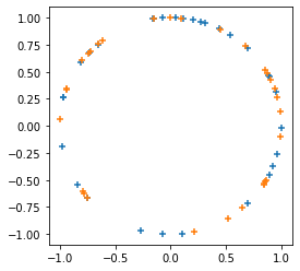
Dodaje tfp.random.sanitize_seed .
Dodaje tfp.random.spherical_uniform .

plt.figure(figsize=(4, 4))
seed = tfp.random.sanitize_seed(123)
seed1, seed2 = tfp.random.split_seed(seed)
samps = tfp.random.spherical_uniform([30], dimension=2, seed=seed1)
plt.scatter(*samps.numpy().T, marker='+')
samps = tfp.random.spherical_uniform([30], dimension=2, seed=seed2)
plt.scatter(*samps.numpy().T, marker='+');

png

Notatnik z informacjami o wersji TFP (0.13.0)

Instalacje i importy

Dystrybucje [matematyka podstawowa]

BetaQuotient

DeterminantalPointProcess

SigmoidBeta

Zipf

NormalInverseGaussian

MatrixNormalLinearOperator

MatrixStudentTLinearOperator

Dystrybucje [oprogramowanie / wrappery]

Sharded

BatchBroadcast

Masked

Bijektory

Restrukturyzacyjne bijektory

Sharded

VI

VI/MAP/MLE

MCMC

init_near_unconstrained_zero , retry_init

Okienkowe adaptacyjne próbniki HMC i NUTS

Matematyka, statystyki

Funkcje Owena T, Erfcx, Logerfc, Logerfcx, Dawson

igammainv / igammacinv

log-kve

Inny

`BetaQuotient`

`DeterminantalPointProcess`

`SigmoidBeta`

`NormalInverseGaussian`

`MatrixNormalLinearOperator`

`MatrixStudentTLinearOperator`

`Sharded`

`BatchBroadcast`

`Masked`

`Sharded`

`init_near_unconstrained_zero` , `retry_init`