احتمالية TensorFlow على JAX

عرض على TensorFlow.org

تشغيل في Google Colab

عرض المصدر على جيثب

تحميل دفتر

TensorFlow الاحتمالية (TFP) هي مكتبة للتفكير والتحليل الإحصائي الاحتمالي الذي يعمل الآن أيضا على JAX ! بالنسبة لأولئك غير المألوفين ، فإن JAX عبارة عن مكتبة للحوسبة الرقمية المتسارعة بناءً على تحويلات الوظائف القابلة للتركيب.

يدعم TFP على JAX الكثير من الوظائف الأكثر فائدة ل TFP العادي مع الحفاظ على التجريدات وواجهات برمجة التطبيقات التي يشعر بها العديد من مستخدمي TFP الآن.

يثبت

TFP على JAX لا تعتمد على TensorFlow. دعنا نلغي تثبيت TensorFlow من Colab بالكامل.

pip uninstall tensorflow -y -q

يمكننا تثبيت TFP على JAX مع أحدث الإصدارات الليلية من TFP.

pip install -Uq tfp-nightly[jax] > /dev/null

دعنا نستورد بعض مكتبات Python المفيدة.

import matplotlib.pyplot as plt
import numpy as np
import seaborn as sns
from sklearn import datasets
sns.set(style='white')

/usr/local/lib/python3.6/dist-packages/statsmodels/tools/_testing.py:19: FutureWarning: pandas.util.testing is deprecated. Use the functions in the public API at pandas.testing instead.
  import pandas.util.testing as tm

دعنا أيضًا نستورد بعض وظائف JAX الأساسية.

import jax.numpy as jnp
from jax import grad
from jax import jit
from jax import random
from jax import value_and_grad
from jax import vmap

استيراد TFP على JAX

لاستخدام TFP على JAX، ببساطة استيراد jax "الركيزة" واستخدامه كما كنت عادة أن tfp :

from tensorflow_probability.substrates import jax as tfp
tfd = tfp.distributions
tfb = tfp.bijectors
tfpk = tfp.math.psd_kernels

العرض التوضيحي: الانحدار اللوجستي Bayesian

لتوضيح ما يمكننا القيام به مع الواجهة الخلفية لـ JAX ، سنقوم بتنفيذ الانحدار اللوجستي Bayesian المطبق على مجموعة بيانات Iris الكلاسيكية.

أولاً ، دعنا نستورد مجموعة بيانات Iris ونستخرج بعض البيانات الوصفية.

iris = datasets.load_iris()
features, labels = iris['data'], iris['target']

num_features = features.shape[-1]
num_classes = len(iris.target_names)

يمكننا تحديد نموذج باستخدام tfd.JointDistributionCoroutine . سوف نضع مقدمو الاديره العادية القياسية على كل من الأوزان وعلى المدى التحيز ثم إرسال target_log_prob الوظيفة التي دبابيس التسميات عينات للبيانات.

Root = tfd.JointDistributionCoroutine.Root
def model():
  w = yield Root(tfd.Sample(tfd.Normal(0., 1.),
                            sample_shape=(num_features, num_classes)))
  b = yield Root(
      tfd.Sample(tfd.Normal(0., 1.), sample_shape=(num_classes,)))
  logits = jnp.dot(features, w) + b
  yield tfd.Independent(tfd.Categorical(logits=logits),
                        reinterpreted_batch_ndims=1)


dist = tfd.JointDistributionCoroutine(model)
def target_log_prob(*params):
  return dist.log_prob(params + (labels,))

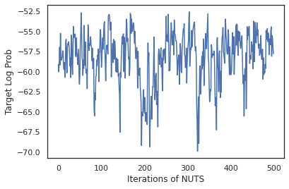
نحن عينة من dist لإنتاج الحالة الأولية للMCMC. يمكننا بعد ذلك تحديد وظيفة تأخذ مفتاحًا عشوائيًا وحالة أولية ، وتنتج 500 عينة من No-U-Turn-Sampler (NUTS). لاحظ أن نتمكن من استخدام التحولات JAX مثل jit لجمع العينات لدينا المكسرات باستخدام XLA.

init_key, sample_key = random.split(random.PRNGKey(0))
init_params = tuple(dist.sample(seed=init_key)[:-1])

@jit
def run_chain(key, state):
  kernel = tfp.mcmc.NoUTurnSampler(target_log_prob, 1e-3)
  return tfp.mcmc.sample_chain(500,
      current_state=state,
      kernel=kernel,
      trace_fn=lambda _, results: results.target_log_prob,
      num_burnin_steps=500,
      seed=key)

states, log_probs = run_chain(sample_key, init_params)
plt.figure()
plt.plot(log_probs)
plt.ylabel('Target Log Prob')
plt.xlabel('Iterations of NUTS')
plt.show()

دعنا نستخدم عيناتنا لإجراء متوسط ​​نموذج بايزي (BMA) عن طريق حساب متوسط ​​الاحتمالات المتوقعة لكل مجموعة من الأوزان.

أولاً ، لنكتب دالة لمجموعة معينة من المعلمات ستنتج الاحتمالات على كل فئة. يمكننا استخدام dist.sample_distributions للحصول على التوزيع النهائي في النموذج.

def classifier_probs(params):
  dists, _ = dist.sample_distributions(seed=random.PRNGKey(0),
                                       value=params + (None,))
  return dists[-1].distribution.probs_parameter()

يمكننا vmap(classifier_probs) على مجموعة من العينات للحصول على الاحتمالات الطبقة توقع لكل من عينات لدينا. ثم نحسب متوسط ​​الدقة عبر كل عينة ، والدقة من متوسط ​​نموذج بايزي.

all_probs = jit(vmap(classifier_probs))(states)
print('Average accuracy:', jnp.mean(all_probs.argmax(axis=-1) == labels))
print('BMA accuracy:', jnp.mean(all_probs.mean(axis=0).argmax(axis=-1) == labels))

Average accuracy: 0.96952
BMA accuracy: 0.97999996

يبدو أن BMA يقلل من معدل الخطأ لدينا بمقدار الثلث تقريبًا!

الأساسيات

TFP على JAX ديه API مطابق لTF حيث بدلا من قبول الأشياء TF مثل tf.Tensor ق أنها تقبل التناظرية JAX. على سبيل المثال، في أي مكان في tf.Tensor كانت تستخدم سابقا المدخلات، وAPI يتوقع الآن JAX DeviceArray . بدلا من إرجاع tf.Tensor ، وأساليب TFP عودة DeviceArray الصورة. يعمل TFP على JAX أيضا مع البنيات المتداخلة من الكائنات JAX، مثل قائمة أو القاموس من DeviceArray الصورة.

التوزيعات

يتم دعم معظم توزيعات TFP في JAX مع دلالات مشابهة جدًا لنظيراتها في فريق العمل. كانت مسجلة أيضا باسم JAX Pytrees ، حتى أنها يمكن أن تكون مدخلات ومخرجات وظائف تحولت JAX.

التوزيعات الأساسية

و log_prob طريقة لتوزيعات يعمل نفس الشيء.

dist = tfd.Normal(0., 1.)
print(dist.log_prob(0.))

-0.9189385

أخذ عينات من توزيع يتطلب اجتياز صراحة في PRNGKey (أو قائمة من الأعداد الصحيحة) مثل seed حجة الكلمة. سيؤدي الفشل في تمرير البذرة بشكل صريح إلى حدوث خطأ.

tfd.Normal(0., 1.).sample(seed=random.PRNGKey(0))

DeviceArray(-0.20584226, dtype=float32)

تبقى دلالات شكل لتوزيعات نفسه في JAX، حيث التوزيعات سوف يكون لها كل event_shape و batch_shape ورسم العديد من العينات سيضيف إضافية sample_shape الأبعاد.

على سبيل المثال، tfd.MultivariateNormalDiag ومع المعلمات ناقلات لها شكل الحدث وناقلات فارغة شكل دفعة واحدة.

dist = tfd.MultivariateNormalDiag(
    loc=jnp.zeros(5),
    scale_diag=jnp.ones(5)
)
print('Event shape:', dist.event_shape)
print('Batch shape:', dist.batch_shape)

Event shape: (5,)
Batch shape: ()

من ناحية أخرى، tfd.Normal معلمات مع ناقلات سيكون لها العددية شكل الحدث وناقلات دفعة الشكل.

dist = tfd.Normal(
    loc=jnp.ones(5),
    scale=jnp.ones(5),
)
print('Event shape:', dist.event_shape)
print('Batch shape:', dist.batch_shape)

Event shape: ()
Batch shape: (5,)

دلالات اتخاذ log_prob العينات تعمل نفس الشيء في JAX جدا.

dist =  tfd.Normal(jnp.zeros(5), jnp.ones(5))
s = dist.sample(sample_shape=(10, 2), seed=random.PRNGKey(0))
print(dist.log_prob(s).shape)

dist =  tfd.Independent(tfd.Normal(jnp.zeros(5), jnp.ones(5)), 1)
s = dist.sample(sample_shape=(10, 2), seed=random.PRNGKey(0))
print(dist.log_prob(s).shape)

(10, 2, 5)
(10, 2)

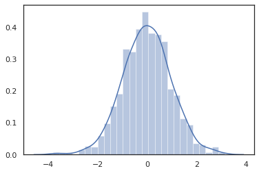
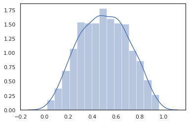
لأن JAX DeviceArray الصورة متوافقة مع مكتبات مثل نمباي وMatplotlib، يمكننا إطعام عينات مباشرة في وظيفة التخطيط.

sns.distplot(tfd.Normal(0., 1.).sample(1000, seed=random.PRNGKey(0)))
plt.show()

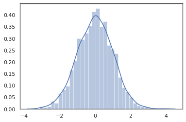
Distribution أساليب متوافقة مع التحولات JAX.

sns.distplot(jit(vmap(lambda key: tfd.Normal(0., 1.).sample(seed=key)))(
    random.split(random.PRNGKey(0), 2000)))
plt.show()

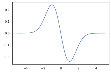
x = jnp.linspace(-5., 5., 100)
plt.plot(x, jit(vmap(grad(tfd.Normal(0., 1.).prob)))(x))
plt.show()

لأن يتم تسجيل توزيعات TFP كعقد pytree JAX، يمكننا كتابة وظائف مع التوزيعات كما المدخلات أو المخرجات وتحويلها باستخدام jit ، لكنها غير معتمدة حتى الآن كوسائط ل vmap ظائف افتتاحية.

@jit
def random_distribution(key):
  loc_key, scale_key = random.split(key)
  loc, log_scale = random.normal(loc_key), random.normal(scale_key)
  return tfd.Normal(loc, jnp.exp(log_scale))
random_dist = random_distribution(random.PRNGKey(0))
print(random_dist.mean(), random_dist.variance())

0.14389051 0.081832744

التوزيعات المتغيرة

توزيعات تحول، أي التوزيعات التي تم تمريرها من خلال عينات Bijector أيضا العمل من خارج منطقة الجزاء (bijectors العمل أيضا! انظر أدناه).

dist = tfd.TransformedDistribution(
    tfd.Normal(0., 1.),
    tfb.Sigmoid()
)
sns.distplot(dist.sample(1000, seed=random.PRNGKey(0)))
plt.show()

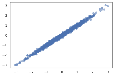
التوزيعات المشتركة

تقدم TFP JointDistribution الصورة لتمكين الجمع بين توزيعات المكونة في توزيع واحد على المتغيرات العشوائية متعددة. حاليا، والعروض TFP ثلاثة متغيرات أساسية ( JointDistributionSequential ، JointDistributionNamed ، و JointDistributionCoroutine ) وجميعها معتمدة في JAX. و AutoBatched كما يدعم جميع المتغيرات.

dist = tfd.JointDistributionSequential([
  tfd.Normal(0., 1.),
  lambda x: tfd.Normal(x, 1e-1)
])
plt.scatter(*dist.sample(1000, seed=random.PRNGKey(0)), alpha=0.5)
plt.show()

joint = tfd.JointDistributionNamed(dict(
    e=             tfd.Exponential(rate=1.),
    n=             tfd.Normal(loc=0., scale=2.),
    m=lambda n, e: tfd.Normal(loc=n, scale=e),
    x=lambda    m: tfd.Sample(tfd.Bernoulli(logits=m), 12),
))
joint.sample(seed=random.PRNGKey(0))

{'e': DeviceArray(3.376818, dtype=float32),
 'm': DeviceArray(2.5449684, dtype=float32),
 'n': DeviceArray(-0.6027825, dtype=float32),
 'x': DeviceArray([1, 1, 1, 1, 1, 1, 1, 1, 1, 1, 1, 1], dtype=int32)}

Root = tfd.JointDistributionCoroutine.Root
def model():
  e = yield Root(tfd.Exponential(rate=1.))
  n = yield Root(tfd.Normal(loc=0, scale=2.))
  m = yield tfd.Normal(loc=n, scale=e)
  x = yield tfd.Sample(tfd.Bernoulli(logits=m), 12)

joint = tfd.JointDistributionCoroutine(model)

joint.sample(seed=random.PRNGKey(0))

StructTuple(var0=DeviceArray(0.17315261, dtype=float32), var1=DeviceArray(-3.290489, dtype=float32), var2=DeviceArray(-3.1949058, dtype=float32), var3=DeviceArray([0, 0, 0, 0, 0, 0, 0, 0, 0, 0, 0, 0], dtype=int32))

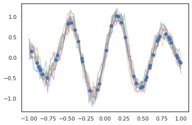
توزيعات أخرى

تعمل عمليات Gaussian أيضًا في وضع JAX!

k1, k2, k3 = random.split(random.PRNGKey(0), 3)
observation_noise_variance = 0.01
f = lambda x: jnp.sin(10*x[..., 0]) * jnp.exp(-x[..., 0]**2)
observation_index_points = random.uniform(
    k1, [50], minval=-1.,maxval= 1.)[..., jnp.newaxis]
observations = f(observation_index_points) + tfd.Normal(
    loc=0., scale=jnp.sqrt(observation_noise_variance)).sample(seed=k2)

index_points = jnp.linspace(-1., 1., 100)[..., jnp.newaxis]

kernel = tfpk.ExponentiatedQuadratic(length_scale=0.1)

gprm = tfd.GaussianProcessRegressionModel(
    kernel=kernel,
    index_points=index_points,
    observation_index_points=observation_index_points,
    observations=observations,
    observation_noise_variance=observation_noise_variance)

samples = gprm.sample(10, seed=k3)
for i in range(10):
  plt.plot(index_points, samples[i], alpha=0.5)
plt.plot(observation_index_points, observations, marker='o', linestyle='')
plt.show()

يتم دعم نماذج ماركوف المخفية أيضًا.

initial_distribution = tfd.Categorical(probs=[0.8, 0.2])
transition_distribution = tfd.Categorical(probs=[[0.7, 0.3],
                                                 [0.2, 0.8]])

observation_distribution = tfd.Normal(loc=[0., 15.], scale=[5., 10.])

model = tfd.HiddenMarkovModel(
    initial_distribution=initial_distribution,
    transition_distribution=transition_distribution,
    observation_distribution=observation_distribution,
    num_steps=7)

print(model.mean())
print(model.log_prob(jnp.zeros(7)))
print(model.sample(seed=random.PRNGKey(0)))

[3.       6.       7.5      8.249999 8.625001 8.812501 8.90625 ]
/usr/local/lib/python3.6/dist-packages/tensorflow_probability/substrates/jax/distributions/hidden_markov_model.py:483: UserWarning: HiddenMarkovModel.log_prob in TFP versions < 0.12.0 had a bug in which the transition model was applied prior to the initial step. This bug has been fixed. You may observe a slight change in behavior.
  'HiddenMarkovModel.log_prob in TFP versions < 0.12.0 had a bug '
-19.855635
[ 1.3641367  0.505798   1.3626463  3.6541772  2.272286  15.10309
 22.794212 ]

هناك عدد قليل من التوزيعات مثل PixelCNN غير معتمدة حتى الآن بسبب تبعيات صارمة على TensorFlow أو XLA عدم التوافق.

باجنز

يتم دعم معظم أجهزة تحفيز TFP في JAX اليوم!

tfb.Exp().inverse(1.)

DeviceArray(0., dtype=float32)

bij = tfb.Shift(1.)(tfb.Scale(3.))
print(bij.forward(jnp.ones(5)))
print(bij.inverse(jnp.ones(5)))

[4. 4. 4. 4. 4.]
[0. 0. 0. 0. 0.]

b = tfb.FillScaleTriL(diag_bijector=tfb.Exp(), diag_shift=None)
print(b.forward(x=[0., 0., 0.]))
print(b.inverse(y=[[1., 0], [.5, 2]]))

[[1. 0.]
 [0. 1.]]
[0.6931472 0.5       0.       ]

b = tfb.Chain([tfb.Exp(), tfb.Softplus()])
# or:
# b = tfb.Exp()(tfb.Softplus())
print(b.forward(-jnp.ones(5)))

[1.3678794 1.3678794 1.3678794 1.3678794 1.3678794]

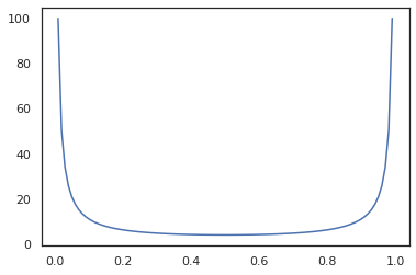
Bijectors تتوافق مع التحولات JAX مثل jit ، grad و vmap .

jit(vmap(tfb.Exp().inverse))(jnp.arange(4.))

DeviceArray([     -inf, 0.       , 0.6931472, 1.0986123], dtype=float32)

x = jnp.linspace(0., 1., 100)
plt.plot(x, jit(grad(lambda x: vmap(tfb.Sigmoid().inverse)(x).sum()))(x))
plt.show()

بعض bijectors، مثل RealNVP و FFJORD غير معتمدة حتى الان.

MCMC

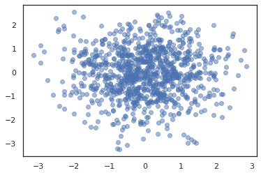
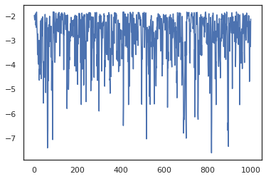
قمنا استدار tfp.mcmc إلى JAX كذلك، حتى نتمكن من تشغيل خوارزميات مثل هاملتون مونت كارلو (HMC) ولا-U-تشغيل-عينات (المكسرات) في JAX.

target_log_prob = tfd.MultivariateNormalDiag(jnp.zeros(2), jnp.ones(2)).log_prob

على عكس TFP على TF، نحن مطالبون تمرير PRNGKey إلى sample_chain باستخدام seed حجة الكلمة.

def run_chain(key, state):
  kernel = tfp.mcmc.NoUTurnSampler(target_log_prob, 1e-1)
  return tfp.mcmc.sample_chain(1000,
      current_state=state,
      kernel=kernel,
      trace_fn=lambda _, results: results.target_log_prob,
      seed=key)
states, log_probs = jit(run_chain)(random.PRNGKey(0), jnp.zeros(2))
plt.figure()
plt.scatter(*states.T, alpha=0.5)
plt.figure()
plt.plot(log_probs)
plt.show()

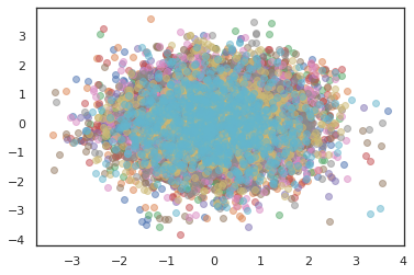
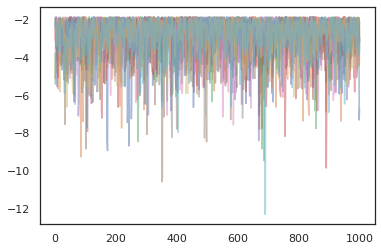
لتشغيل سلاسل متعددة، يمكننا إما تمرير مجموعة من الدول في sample_chain أو استخدام vmap (على الرغم من أننا لم تستكشف بعد الاختلافات الأداء بين النهجين).

states, log_probs = jit(run_chain)(random.PRNGKey(0), jnp.zeros([10, 2]))
plt.figure()
for i in range(10):
  plt.scatter(*states[:, i].T, alpha=0.5)
plt.figure()
for i in range(10):
  plt.plot(log_probs[:, i], alpha=0.5)
plt.show()

محسنون

يدعم TFP على JAX بعض المحسّنات المهمة مثل BFGS و L-BFGS. لنقم بإعداد دالة خسارة تربيعية متدرجة بسيطة.

minimum = jnp.array([1.0, 1.0])  # The center of the quadratic bowl.
scales = jnp.array([2.0, 3.0])  # The scales along the two axes.

# The objective function and the gradient.
def quadratic_loss(x):
  return jnp.sum(scales * jnp.square(x - minimum))

start = jnp.array([0.6, 0.8])  # Starting point for the search.

يمكن لـ BFGS إيجاد الحد الأدنى من هذه الخسارة.

optim_results = tfp.optimizer.bfgs_minimize(
    value_and_grad(quadratic_loss), initial_position=start, tolerance=1e-8)

# Check that the search converged
assert(optim_results.converged)
# Check that the argmin is close to the actual value.
np.testing.assert_allclose(optim_results.position, minimum)
# Print out the total number of function evaluations it took. Should be 5.
print("Function evaluations: %d" % optim_results.num_objective_evaluations)

Function evaluations: 5

لذلك يمكن لـ L-BFGS.

optim_results = tfp.optimizer.lbfgs_minimize(
    value_and_grad(quadratic_loss), initial_position=start, tolerance=1e-8)

# Check that the search converged
assert(optim_results.converged)
# Check that the argmin is close to the actual value.
np.testing.assert_allclose(optim_results.position, minimum)
# Print out the total number of function evaluations it took. Should be 5.
print("Function evaluations: %d" % optim_results.num_objective_evaluations)

Function evaluations: 5

ل vmap L-BFGS، دعونا مجموعة لتصل إلى وظيفة أن يحسن خسارة نقطة انطلاق واحدة.

def optimize_single(start):
  return tfp.optimizer.lbfgs_minimize(
      value_and_grad(quadratic_loss), initial_position=start, tolerance=1e-8)

all_results = jit(vmap(optimize_single))(
    random.normal(random.PRNGKey(0), (10, 2)))
assert all(all_results.converged)
for i in range(10):
  np.testing.assert_allclose(optim_results.position[i], minimum)
print("Function evaluations: %s" % all_results.num_objective_evaluations)

Function evaluations: [6 6 9 6 6 8 6 8 5 9]

تحفظات

هناك بعض الاختلافات الأساسية بين TF و JAX ، وستكون بعض سلوكيات TFP مختلفة بين الركيزتين ولا يتم دعم جميع الوظائف. فمثلا،

• TFP على JAX لا يدعم أي شيء مثل tf.Variable منذ شيء مثل ذلك موجود في JAX. وهذا يعني أيضا المرافق مثل tfp.util.TransformedVariable غير معتمدة سواء.
• tfp.layers غير معتمد في الخلفية بعد، نظرا لاعتمادها على Keras و tf.Variable الصورة.
• tfp.math.minimize لا يعمل في TFP على JAX بسبب اعتمادها على tf.Variable .
• باستخدام TFP على JAX ، تكون أشكال الموتر دائمًا قيمًا صحيحة محددة وغير معروفة / ديناميكية أبدًا كما هو الحال في TFP على TF.
• يتم التعامل مع العشوائية الزائفة بشكل مختلف في TF و JAX (انظر الملحق).
• المكتبات في tfp.experimental ليست مضمونة في الوجود في الركيزة JAX.
• تختلف قواعد الترويج لـ Dtype بين TF و JAX. يحاول TFP في JAX احترام دلالات نوع dtype داخليًا ، من أجل الاتساق.
• لم يتم تسجيل Bijectors على أنها pytrees JAX.

للاطلاع على القائمة الكاملة لما معتمد في TFP على JAX، يرجى الرجوع إلى وثائق API .

استنتاج

لقد نقلنا الكثير من ميزات TFP إلى JAX ونحن متحمسون لمعرفة ما سيبنيه الجميع. بعض الوظائف غير مدعومة حتى الآن ؛ إذا كنا قد غاب عن شيء مهم بالنسبة لك (أو إذا وجدت علة!) يرجى التواصل معنا - يمكنك البريد الإلكتروني tfprobability@tensorflow.org أو ملف قضية على لدينا الريبو جيثب .

الملحق: العشوائية الزائفة في JAX

الجيل عدد المزيف (PRNG) نموذج JAX هو عديمي الجنسية. على عكس نموذج الحالة ، لا توجد حالة عالمية قابلة للتغيير تتطور بعد كل رسم عشوائي. في نموذج JAX، ونبدأ مع مفتاح PRNG، الذي يعمل بمثابة زوج من الأعداد الصحيحة 32-بت. يمكننا بناء هذه المفاتيح باستخدام jax.random.PRNGKey .

key = random.PRNGKey(0)  # Creates a key with value [0, 0]
print(key)

[0 0]

وظائف عشوائية في JAX تستهلك مفتاح لإنتاج حتمي لVARIATE عشوائي، وهذا يعني أنها لا ينبغي أن تستخدم مرة أخرى. على سبيل المثال، يمكننا استخدام key لعينة قيمة توزع عادة، ولكن لا ينبغي لنا أن استخدام key مرة أخرى في مكان آخر. وعلاوة على ذلك، ويمر نفس القيمة في random.normal سوف تنتج نفس القيمة.

print(random.normal(key))

-0.20584226

إذن كيف يمكننا سحب عينات متعددة من مفتاح واحد؟ الجواب هو تقسيم الرئيسي. والفكرة الأساسية هي أن نتمكن من تقسيم PRNGKey الى عدة، ويمكن التعامل مع كل من مفاتيح جديدة ومصدر مستقل من العشوائية.

key1, key2 = random.split(key, num=2)
print(key1, key2)

[4146024105  967050713] [2718843009 1272950319]

يعد تقسيم المفتاح أمرًا حتميًا ولكنه فوضوي ، لذلك يمكن الآن استخدام كل مفتاح جديد لرسم عينة عشوائية مميزة.

print(random.normal(key1), random.normal(key2))

0.14389051 -1.2515389

لمزيد من المعلومات حول نموذج مفتاح تقسيم حتمية JAX، انظر هذا الدليل .