| | |  عرض المصدر على جيثب عرض المصدر على جيثب | |
هذا منفذ احتمالية TensorFlow للورقة التي تحمل نفس الاسم بتاريخ 16 مارس 2020 بواسطة Li et al. نحن نعيد إنتاج أساليب المؤلفين الأصليين ونتائجهم بأمانة على منصة احتمالية TensorFlow ، حيث نعرض بعض قدرات TFP في إعداد نمذجة علم الأوبئة الحديثة. يمنحنا النقل إلى TensorFlow تسريعًا يقارب 10 مرات بالنسبة إلى كود Matlab الأصلي ، وبما أن TensorFlow Probability يدعم بشكل واسع حساب الدُفعات الموجهة ، فإنه يتسع أيضًا بشكل إيجابي لمئات التكرارات المستقلة.
الورقة الأصلية
Ruiyun Li و Sen Pei و Bin Chen و Yimeng Song و Tao Zhang و Wan Yang و Jeffrey Shaman. تسهل العدوى الجسيمة غير الموثقة الانتشار السريع لفيروس كورونا الجديد (SARS-CoV2). (2020)، دوى: https://doi.org/10.1126/science.abb3221 .
الخلاصة: "تقدير مدى انتشار والإعداء من الالتهابات غير موثقة التاجى رواية (SARS-CoV2) أمر بالغ الأهمية لفهم انتشار الشامل والقدرة على إحداث جائحة من هذا المرض هنا نستخدم الملاحظات الإصابة المبلغ عنها داخل الصين، جنبا إلى جنب مع بيانات التنقل، و نموذج التمثيل الغذائي الديناميكي المتصل بالشبكة والاستدلال البايزي ، لاستنتاج الخصائص الوبائية الحرجة المرتبطة بـ SARS-CoV2 ، بما في ذلك جزء من العدوى غير الموثقة ومعدلاتها. نقدر أن 86٪ من جميع الإصابات كانت غير موثقة (95٪ CI: [82٪ - 90٪] ) قبل 23 يناير 2020. قيود السفر لكل شخص ، كان معدل انتقال العدوى غير الموثقة 55٪ من الإصابات الموثقة ([46٪ -62٪]) ، ومع ذلك ، نظرًا لأعدادهم الكبيرة ، كانت العدوى غير الموثقة مصدر العدوى لـ 79 النسبة المئوية للحالات الموثقة. تشرح هذه النتائج الانتشار الجغرافي السريع لـ SARS-CoV2 وتشير إلى أن احتواء هذا الفيروس سيكون صعبًا بشكل خاص. "
جيثب تصل إلى التعليمات البرمجية والبيانات.
ملخص
والنموذج هو نموذج المرض المجزئ ، مع مقصورات ل "عرضة"، "يتعرض" (مصاب ولكن ليس معديا بعد)، "موثقة أبدا المعدية"، و "وثقت في نهاية المطاف المعدية". هناك ميزتان جديرتان بالملاحظة: مقصورات منفصلة لكل مدينة من 375 مدينة صينية ، مع افتراض حول كيفية انتقال الناس من مدينة إلى أخرى ؛ والتأخير في الإبلاغ عن الإصابة، بحيث الحالة التي يصبح "وثقت في نهاية المطاف المعدية" في يوم \(t\) لا تظهر في التهم حالة المرصودة حتى اليوم في وقت لاحق العشوائية.
يفترض النموذج أن الحالات التي لم يتم توثيقها مطلقًا تنتهي بعدم توثيقها بكونها أكثر اعتدالًا ، وبالتالي تصيب الآخرين بمعدل أقل. المعلمة الرئيسية للاهتمام في الورقة الأصلية هي نسبة الحالات التي لا يتم توثيقها ، لتقدير كل من مدى العدوى الموجودة ، وتأثير الانتقال غير الموثق على انتشار المرض.
تم تصميم هذا الكولاب باعتباره تجولًا في الكود بأسلوب تصاعدي. بالترتيب ، سنفعل
- استيعاب البيانات وفحصها بإيجاز ،
- تحديد مساحة الدولة وديناميكيات النموذج ،
- قم ببناء مجموعة من الوظائف للقيام بالاستدلال في النموذج الذي يتبع Li et al ، و
- ادعهم وافحص النتائج. المفسد: يخرجون مثل الورق.
التثبيت وواردات بايثون
pip3 install -q tf-nightly tfp-nightly
import collections
import io
import requests
import time
import zipfile

import matplotlib.pyplot as plt
import numpy as np
import pandas as pd

import tensorflow.compat.v2 as tf
import tensorflow_probability as tfp
from tensorflow_probability.python.internal import samplers

tfd = tfp.distributions
tfes = tfp.experimental.sequential
استيراد البيانات
دعنا نستورد البيانات من جيثب ونفحص بعضها.
r = requests.get('https://raw.githubusercontent.com/SenPei-CU/COVID-19/master/Data.zip')
z = zipfile.ZipFile(io.BytesIO(r.content))
z.extractall('/tmp/')
raw_incidence = pd.read_csv('/tmp/data/Incidence.csv')
raw_mobility = pd.read_csv('/tmp/data/Mobility.csv')
raw_population = pd.read_csv('/tmp/data/pop.csv')
أدناه يمكننا أن نرى عدد الوقوع الخام في اليوم. نحن مهتمون أكثر في أول 14 يومًا (10 يناير إلى 23 يناير) ، حيث تم وضع قيود السفر في 23 يناير. تتعامل الورقة مع هذا من خلال نمذجة 10-23 يناير و 23 يناير + بشكل منفصل ، مع معلمات مختلفة ؛ سنقتصر إعادة إنتاجنا على الفترة السابقة فقط.
raw_incidence.drop('Date', axis=1)  # The 'Date' column is all 1/18/21
# Luckily the days are in order, starting on January 10th, 2020.
دعونا نتحقق من صحة عدد حالات الإصابة في ووهان.
plt.plot(raw_incidence.Wuhan, '.-')
plt.title('Wuhan incidence counts over 1/10/20 - 02/08/20')
plt.show()
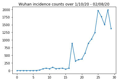
حتى الان جيدة جدا. الآن يتم حساب عدد السكان الأولي.
raw_population
دعنا أيضًا نتحقق ونسجل أي إدخال هو ووهان.
raw_population['City'][169]
'Wuhan'
WUHAN_IDX = 169
وهنا نرى مصفوفة التنقل بين المدن المختلفة. هذا وكيل لعدد الأشخاص الذين يتنقلون بين المدن المختلفة في أول 14 يومًا. إنه محفور من سجلات GPS التي قدمتها Tencent لموسم العام القمري الجديد 2018. لي وآخرون نموذج التنقل خلال موسم 2020 وبعض المجهول (رهنا الاستدلال) عاملا ثابتا \(\theta\) مرات هذا.
raw_mobility
أخيرًا ، دعنا نعالج كل هذا مسبقًا في مصفوفات عددية يمكننا استهلاكها.
# The given populations are only "initial" because of intercity mobility during
# the holiday season.
initial_population = raw_population['Population'].to_numpy().astype(np.float32)
قم بتحويل بيانات التنقل إلى موتر على شكل [L ، L ، T] ، حيث L هو عدد المواقع ، و T هو عدد الخطوات الزمنية.
daily_mobility_matrices = []
for i in range(1, 15):
  day_mobility = raw_mobility[raw_mobility['Day'] == i]

  # Make a matrix of daily mobilities.
  z = pd.crosstab(
      day_mobility.Origin,
      day_mobility.Destination,
      values=day_mobility['Mobility Index'], aggfunc='sum', dropna=False)

  # Include every city, even if there are no rows for some in the raw data on
  # some day.  This uses the sort order of `raw_population`.
  z = z.reindex(index=raw_population['City'], columns=raw_population['City'],
                fill_value=0)
  # Finally, fill any missing entries with 0. This means no mobility.
  z = z.fillna(0)
  daily_mobility_matrices.append(z.to_numpy())

mobility_matrix_over_time = np.stack(daily_mobility_matrices, axis=-1).astype(
    np.float32)
أخيرًا ، خذ الإصابات الملحوظة وقم بعمل جدول [L ، T].
# Remove the date parameter and take the first 14 days.
observed_daily_infectious_count = raw_incidence.to_numpy()[:14, 1:]
observed_daily_infectious_count = np.transpose(
    observed_daily_infectious_count).astype(np.float32)
وتحقق مرة أخرى من أننا حصلنا على الأشكال بالطريقة التي أردناها. للتذكير ، نحن نعمل مع 375 مدينة و 14 يومًا.
print('Mobility Matrix over time should have shape (375, 375, 14): {}'.format(
    mobility_matrix_over_time.shape))
print('Observed Infectious should have shape (375, 14): {}'.format(
    observed_daily_infectious_count.shape))
print('Initial population should have shape (375): {}'.format(
    initial_population.shape))
Mobility Matrix over time should have shape (375, 375, 14): (375, 375, 14)
Observed Infectious should have shape (375, 14): (375, 14)
Initial population should have shape (375): (375,)
تحديد الحالة والمعلمات
لنبدأ في تحديد نموذجنا. إن النموذج الذي يتم استنساخ هو البديل ل نموذج سعير . في هذه الحالة ، لدينا الحالات التالية المتغيرة بمرور الوقت:
- \(S\): عدد الأشخاص المعرضين لهذا المرض في كل مدينة.
- \(E\): عدد الأشخاص في كل مدينة تتعرض لهذا المرض ولكن ليس معديا حتى الان. من الناحية البيولوجية ، هذا يتوافق مع الإصابة بالمرض ، حيث يصبح جميع الأشخاص المعرضين للعدوى في النهاية.
- \(I^u\): عدد الأشخاص في كل مدينة وهم معدية لكنها لا يحملون وثائق. في النموذج ، هذا يعني في الواقع "لن يتم توثيقه أبدًا".
- \(I^r\): عدد الأشخاص في كل مدينة وهم المعدية وموثقة على هذا النحو. لي وآخرون نموذج التأخير التقارير، لذلك \(I^r\) يناظر شيء من هذا القبيل "القضية هي ما يكفي قاسية لتكون موثقة في مرحلة ما في المستقبل".
كما سنرى أدناه ، سنستنتج هذه الحالات عن طريق تشغيل مرشح كالمان المعدل (EAKF) في الوقت المناسب. متجه الحالة لـ EAKF هو ناقل واحد مفهرس حسب المدينة لكل من هذه الكميات.
يحتوي النموذج على المعلمات العالمية غير المتغيرة الزمنية التالية التي لا يمكن الاستدلال عليها:
- \(\beta\): معدل انتقال الأفراد بسبب المعدية موثقة.
- \(\mu\): معدل انتقال النسبي نظرا لأفراد لا يحملون وثائق المعدية. وهذا التصرف من خلال المنتج \(\mu \beta\).
- \(\theta\): العامل بين المدن التنقل. هذا عامل أكبر من 1 لتصحيح نقص الإبلاغ عن بيانات التنقل (والنمو السكاني من 2018 إلى 2020).
- \(Z\): متوسط فترة الحضانة (أي وقت في ولاية "يتعرض").
- \(\alpha\): هذا هو جزء من التهابات شديدة بما يكفي لتكون (النهاية) موثقة.
- \(D\): متوسط مدة العدوى (أي وقت في أي دولة "المعدية").
سنستنتج تقديرات النقاط لهذه المعلمات بحلقة تصفية تكرارية حول EAKF للحالات.
يعتمد النموذج أيضًا على الثوابت غير المستنبطة:
- \(M\): المصفوفة بين المدن التنقل. هذا متغير بمرور الوقت ومن المفترض أنه معطى. أذكر هذا ما تحجيمها من قبل الاستدلال المعلمة \(\theta\) لإعطاء تحركات السكان الفعلية بين المدن.
- \(N\): إن العدد الإجمالي للأشخاص في كل مدينة. يتم أخذ السكان الأولي على النحو الوارد، ويتم احتساب الفترة الزمنية الاختلاف من السكان من التنقل أرقام \(\theta M\).
أولاً ، نعطي أنفسنا بعض هياكل البيانات للاحتفاظ بحالاتنا ومعلماتنا.
SEIRComponents = collections.namedtuple(
  typename='SEIRComponents',
  field_names=[
    'susceptible',              # S
    'exposed',                  # E
    'documented_infectious',    # I^r
    'undocumented_infectious',  # I^u
    # This is the count of new cases in the "documented infectious" compartment.
    # We need this because we will introduce a reporting delay, between a person
    # entering I^r and showing up in the observable case count data.
    # This can't be computed from the cumulative `documented_infectious` count,
    # because some portion of that population will move to the 'recovered'
    # state, which we aren't tracking explicitly.
    'daily_new_documented_infectious'])

ModelParams = collections.namedtuple(
    typename='ModelParams',
    field_names=[
      'documented_infectious_tx_rate',             # Beta
      'undocumented_infectious_tx_relative_rate',  # Mu
      'intercity_underreporting_factor',           # Theta
      'average_latency_period',                    # Z
      'fraction_of_documented_infections',         # Alpha
      'average_infection_duration'                 # D
    ]
)
نقوم أيضًا بترميز حدود Li et al لقيم المعلمات.
PARAMETER_LOWER_BOUNDS = ModelParams(
    documented_infectious_tx_rate=0.8,
    undocumented_infectious_tx_relative_rate=0.2,
    intercity_underreporting_factor=1.,
    average_latency_period=2.,
    fraction_of_documented_infections=0.02,
    average_infection_duration=2.
)

PARAMETER_UPPER_BOUNDS = ModelParams(
    documented_infectious_tx_rate=1.5,
    undocumented_infectious_tx_relative_rate=1.,
    intercity_underreporting_factor=1.75,
    average_latency_period=5.,
    fraction_of_documented_infections=1.,
    average_infection_duration=5.
)
ديناميكيات SEIR
هنا نحدد العلاقة بين المعلمات والحالة.
معادلات ديناميكا الوقت من Li et al (المواد التكميلية ، eqns 1-5) هي كما يلي:
\(\frac{dS_i}{dt} = -\beta \frac{S_i I_i^r}{N_i} - \mu \beta \frac{S_i I_i^u}{N_i} + \theta \sum_k \frac{M_{ij} S_j}{N_j - I_j^r} - + \theta \sum_k \frac{M_{ji} S_j}{N_i - I_i^r}\)
\(\frac{dE_i}{dt} = \beta \frac{S_i I_i^r}{N_i} + \mu \beta \frac{S_i I_i^u}{N_i} -\frac{E_i}{Z} + \theta \sum_k \frac{M_{ij} E_j}{N_j - I_j^r} - + \theta \sum_k \frac{M_{ji} E_j}{N_i - I_i^r}\)
\(\frac{dI^r_i}{dt} = \alpha \frac{E_i}{Z} - \frac{I_i^r}{D}\)
\(\frac{dI^u_i}{dt} = (1 - \alpha) \frac{E_i}{Z} - \frac{I_i^u}{D} + \theta \sum_k \frac{M_{ij} I_j^u}{N_j - I_j^r} - + \theta \sum_k \frac{M_{ji} I^u_j}{N_i - I_i^r}\)
\(N_i = N_i + \theta \sum_j M_{ij} - \theta \sum_j M_{ji}\)
وللتذكير، فإن \(i\) و \(j\) المدن مؤشر السفلية. تمثل هذه المعادلات نموذجًا للتطور الزمني للمرض من خلاله
- الاتصال مع الأفراد المصابين بالعدوى مما يؤدي إلى مزيد من العدوى ؛
- تطور المرض من "المعرض" إلى إحدى الحالات "المعدية" ؛
- تطور المرض من الحالات "المعدية" إلى التعافي ، وهو ما نمثله بالإزالة من السكان النموذجيين ؛
- التنقل بين المدن ، بما في ذلك الأشخاص المصابون بالعدوى المعرضين أو غير المسجلين ؛ و
- التباين الزمني لسكان المدينة اليوميين من خلال التنقل بين المدن.
باتباع Li et al ، نفترض أن الأشخاص الذين يعانون من الحالات الشديدة بدرجة كافية ليتم الإبلاغ عنها في النهاية لا يسافرون بين المدن.
باتباع Li et al أيضًا ، نتعامل مع هذه الديناميكيات على أنها خاضعة لضوضاء Poisson المصطلح ، أي أن كل مصطلح هو في الواقع معدل Poisson ، عينة من التي تعطي التغيير الحقيقي. تعد ضوضاء بواسون من الحكمة لأن طرح عينات بواسون (بدلاً من الإضافة) لا ينتج عنه نتيجة موزعة بواسون.
سنطور هذه الديناميكيات إلى الأمام في الوقت المناسب باستخدام أداة دمج Runge-Kutta الكلاسيكية من الدرجة الرابعة ، ولكن دعونا أولاً نحدد الوظيفة التي تحسبها (بما في ذلك أخذ عينات من ضوضاء بواسون).
def sample_state_deltas(
    state, population, mobility_matrix, params, seed, is_deterministic=False):
  """Computes one-step change in state, including Poisson sampling.

  Note that this is coded to support vectorized evaluation on arbitrary-shape
  batches of states.  This is useful, for example, for running multiple
  independent replicas of this model to compute credible intervals for the
  parameters.  We refer to the arbitrary batch shape with the conventional
  `B` in the parameter documentation below.  This function also, of course,
  supports broadcasting over the batch shape.

  Args:
    state: A `SEIRComponents` tuple with fields Tensors of shape
      B + [num_locations] giving the current disease state.
    population: A Tensor of shape B + [num_locations] giving the current city
      populations.
    mobility_matrix: A Tensor of shape B + [num_locations, num_locations] giving
      the current baseline inter-city mobility.
    params: A `ModelParams` tuple with fields Tensors of shape B giving the
      global parameters for the current EAKF run.
    seed: Initial entropy for pseudo-random number generation.  The Poisson
      sampling is repeatable by supplying the same seed.
    is_deterministic: A `bool` flag to turn off Poisson sampling if desired.

  Returns:
    delta: A `SEIRComponents` tuple with fields Tensors of shape
      B + [num_locations] giving the one-day changes in the state, according
      to equations 1-4 above (including Poisson noise per Li et al).
  """
  undocumented_infectious_fraction = state.undocumented_infectious / population
  documented_infectious_fraction = state.documented_infectious / population

  # Anyone not documented as infectious is considered mobile
  mobile_population = (population - state.documented_infectious)
  def compute_outflow(compartment_population):
    raw_mobility = tf.linalg.matvec(
        mobility_matrix, compartment_population / mobile_population)
    return params.intercity_underreporting_factor * raw_mobility
  def compute_inflow(compartment_population):
    raw_mobility = tf.linalg.matmul(
        mobility_matrix,
        (compartment_population / mobile_population)[..., tf.newaxis],
        transpose_a=True)
    return params.intercity_underreporting_factor * tf.squeeze(
        raw_mobility, axis=-1)

  # Helper for sampling the Poisson-variate terms.
  seeds = samplers.split_seed(seed, n=11)
  if is_deterministic:
    def sample_poisson(rate):
      return rate
  else:
    def sample_poisson(rate):
      return tfd.Poisson(rate=rate).sample(seed=seeds.pop())

  # Below are the various terms called U1-U12 in the paper. We combined the
  # first two, which should be fine; both are poisson so their sum is too, and
  # there's no risk (as there could be in other terms) of going negative.
  susceptible_becoming_exposed = sample_poisson(
      state.susceptible *
      (params.documented_infectious_tx_rate *
       documented_infectious_fraction +
       (params.undocumented_infectious_tx_relative_rate *
        params.documented_infectious_tx_rate) *
       undocumented_infectious_fraction))  # U1 + U2

  susceptible_population_inflow = sample_poisson(
      compute_inflow(state.susceptible))  # U3
  susceptible_population_outflow = sample_poisson(
      compute_outflow(state.susceptible))  # U4

  exposed_becoming_documented_infectious = sample_poisson(
      params.fraction_of_documented_infections *
      state.exposed / params.average_latency_period)  # U5
  exposed_becoming_undocumented_infectious = sample_poisson(
      (1 - params.fraction_of_documented_infections) *
      state.exposed / params.average_latency_period)  # U6

  exposed_population_inflow = sample_poisson(
      compute_inflow(state.exposed))  # U7
  exposed_population_outflow = sample_poisson(
      compute_outflow(state.exposed))  # U8

  documented_infectious_becoming_recovered = sample_poisson(
      state.documented_infectious /
      params.average_infection_duration)  # U9
  undocumented_infectious_becoming_recovered = sample_poisson(
      state.undocumented_infectious /
      params.average_infection_duration)  # U10

  undocumented_infectious_population_inflow = sample_poisson(
      compute_inflow(state.undocumented_infectious))  # U11
  undocumented_infectious_population_outflow = sample_poisson(
      compute_outflow(state.undocumented_infectious))  # U12

  # The final state_deltas
  return SEIRComponents(
      # Equation [1]
      susceptible=(-susceptible_becoming_exposed +
                   susceptible_population_inflow +
                   -susceptible_population_outflow),
      # Equation [2]
      exposed=(susceptible_becoming_exposed +
               -exposed_becoming_documented_infectious +
               -exposed_becoming_undocumented_infectious +
               exposed_population_inflow +
               -exposed_population_outflow),
      # Equation [3]
      documented_infectious=(
          exposed_becoming_documented_infectious +
          -documented_infectious_becoming_recovered),
      # Equation [4]
      undocumented_infectious=(
          exposed_becoming_undocumented_infectious +
          -undocumented_infectious_becoming_recovered +
          undocumented_infectious_population_inflow +
          -undocumented_infectious_population_outflow),
      # New to-be-documented infectious cases, subject to the delayed
      # observation model.
      daily_new_documented_infectious=exposed_becoming_documented_infectious)
ها هو المُتكامل. هذا هو المعيار تماما، باستثناء تمرير البذور PRNG من خلال ل sample_state_deltas تعمل للحصول على الضوضاء بواسون مستقل في كل خطوة من الخطوات الجزئية التي المكالمات طريقة رونج كوتا لل.
@tf.function(autograph=False)
def rk4_one_step(state, population, mobility_matrix, params, seed):
  """Implement one step of RK4, wrapped around a call to sample_state_deltas."""
  # One seed for each RK sub-step
  seeds = samplers.split_seed(seed, n=4)

  deltas = tf.nest.map_structure(tf.zeros_like, state)
  combined_deltas = tf.nest.map_structure(tf.zeros_like, state)

  for a, b in zip([1., 2, 2, 1.], [6., 3., 3., 6.]):
    next_input = tf.nest.map_structure(
        lambda x, delta, a=a: x + delta / a, state, deltas)
    deltas = sample_state_deltas(
        next_input,
        population,
        mobility_matrix,
        params,
        seed=seeds.pop(), is_deterministic=False)
    combined_deltas = tf.nest.map_structure(
        lambda x, delta, b=b: x + delta / b, combined_deltas, deltas)

  return tf.nest.map_structure(
      lambda s, delta: s + tf.round(delta),
      state, combined_deltas)
التهيئة
هنا نقوم بتنفيذ مخطط التهيئة من الورقة.
بعد Li et al ، سيكون مخطط الاستدلال الخاص بنا عبارة عن حلقة داخلية لفلتر كالمان لتعديل المجموعة ، محاطة بحلقة خارجية متكررة للترشيح (IF-EAKF). من الناحية الحسابية ، هذا يعني أننا بحاجة إلى ثلاثة أنواع من التهيئة:
- الحالة الأولية لـ EAKF الداخلي
- المعلمات الأولية لـ IF الخارجي ، وهي أيضًا المعلمات الأولية لـ EAKF الأول
- تحديث المعلمات من تكرار IF إلى التالي ، والتي تعمل كمعلمات أولية لكل EAKF بخلاف الأول.
def initialize_state(num_particles, num_batches, seed):
  """Initialize the state for a batch of EAKF runs.

  Args:
    num_particles: `int` giving the number of particles for the EAKF.
    num_batches: `int` giving the number of independent EAKF runs to
      initialize in a vectorized batch.
    seed: PRNG entropy.

  Returns:
    state: A `SEIRComponents` tuple with Tensors of shape [num_particles,
      num_batches, num_cities] giving the initial conditions in each
      city, in each filter particle, in each batch member.
  """
  num_cities = mobility_matrix_over_time.shape[-2]
  state_shape = [num_particles, num_batches, num_cities]
  susceptible = initial_population * np.ones(state_shape, dtype=np.float32)
  documented_infectious = np.zeros(state_shape, dtype=np.float32)
  daily_new_documented_infectious = np.zeros(state_shape, dtype=np.float32)

  # Following Li et al, initialize Wuhan with up to 2000 people exposed
  # and another up to 2000 undocumented infectious.
  rng = np.random.RandomState(seed[0] % (2**31 - 1))
  wuhan_exposed = rng.randint(
      0, 2001, [num_particles, num_batches]).astype(np.float32)
  wuhan_undocumented_infectious = rng.randint(
      0, 2001, [num_particles, num_batches]).astype(np.float32)

  # Also following Li et al, initialize cities adjacent to Wuhan with three
  # days' worth of additional exposed and undocumented-infectious cases,
  # as they may have traveled there before the beginning of the modeling
  # period.
  exposed = 3 * mobility_matrix_over_time[
      WUHAN_IDX, :, 0] * wuhan_exposed[
          ..., np.newaxis] / initial_population[WUHAN_IDX]
  undocumented_infectious = 3 * mobility_matrix_over_time[
      WUHAN_IDX, :, 0] * wuhan_undocumented_infectious[
          ..., np.newaxis] / initial_population[WUHAN_IDX]

  exposed[..., WUHAN_IDX] = wuhan_exposed
  undocumented_infectious[..., WUHAN_IDX] = wuhan_undocumented_infectious

  # Following Li et al, we do not remove the inital exposed and infectious
  # persons from the susceptible population.
  return SEIRComponents(
      susceptible=tf.constant(susceptible),
      exposed=tf.constant(exposed),
      documented_infectious=tf.constant(documented_infectious),
      undocumented_infectious=tf.constant(undocumented_infectious),
      daily_new_documented_infectious=tf.constant(daily_new_documented_infectious))

def initialize_params(num_particles, num_batches, seed):
  """Initialize the global parameters for the entire inference run.

  Args:
    num_particles: `int` giving the number of particles for the EAKF.
    num_batches: `int` giving the number of independent EAKF runs to
      initialize in a vectorized batch.
    seed: PRNG entropy.

  Returns:
    params: A `ModelParams` tuple with fields Tensors of shape
      [num_particles, num_batches] giving the global parameters
      to use for the first batch of EAKF runs.
  """
  # We have 6 parameters. We'll initialize with a Sobol sequence,
  # covering the hyper-rectangle defined by our parameter limits.
  halton_sequence = tfp.mcmc.sample_halton_sequence(
      dim=6, num_results=num_particles * num_batches, seed=seed)
  halton_sequence = tf.reshape(
      halton_sequence, [num_particles, num_batches, 6])
  halton_sequences = tf.nest.pack_sequence_as(
      PARAMETER_LOWER_BOUNDS, tf.split(
          halton_sequence, num_or_size_splits=6, axis=-1))
  def interpolate(minval, maxval, h):
    return (maxval - minval) * h + minval
  return tf.nest.map_structure(
      interpolate,
      PARAMETER_LOWER_BOUNDS, PARAMETER_UPPER_BOUNDS, halton_sequences)

def update_params(num_particles, num_batches,
                  prev_params, parameter_variance, seed):
  """Update the global parameters between EAKF runs.

  Args:
    num_particles: `int` giving the number of particles for the EAKF.
    num_batches: `int` giving the number of independent EAKF runs to
      initialize in a vectorized batch.
    prev_params: A `ModelParams` tuple of the parameters used for the previous
      EAKF run.
    parameter_variance: A `ModelParams` tuple specifying how much to drift
      each parameter.
    seed: PRNG entropy.

  Returns:
    params: A `ModelParams` tuple with fields Tensors of shape
      [num_particles, num_batches] giving the global parameters
      to use for the next batch of EAKF runs.
  """
  # Initialize near the previous set of parameters. This is the first step
  # in Iterated Filtering.
  seeds = tf.nest.pack_sequence_as(
      prev_params, samplers.split_seed(seed, n=len(prev_params)))
  return tf.nest.map_structure(
      lambda x, v, seed: x + tf.math.sqrt(v) * tf.random.stateless_normal([
          num_particles, num_batches, 1], seed=seed),
      prev_params, parameter_variance, seeds)
التأخير
تتمثل إحدى السمات المهمة لهذا النموذج في الأخذ في الاعتبار بوضوح حقيقة أن العدوى يتم الإبلاغ عنها في وقت متأخر عن بدايتها. وهذا هو، فإننا نتوقع أن الشخص الذي ينتقل من \(E\) مقصورة على \(I^r\) مقصورة على يوم \(t\) قد لا تظهر في ملاحظتها التهم حالة المبلغ عنها حتى في يوم من الأيام في وقت لاحق.
نحن نفترض أن التأخير موزع بأشعة غاما. باتباع Li et al ، نستخدم 1.85 للشكل ، ونضع معلمات للمعدل لإنتاج متوسط تأخير للتقرير يبلغ 9 أيام.
def raw_reporting_delay_distribution(gamma_shape=1.85, reporting_delay=9.):
  return tfp.distributions.Gamma(
      concentration=gamma_shape, rate=gamma_shape / reporting_delay)
ملاحظاتنا منفصلة ، لذلك سنقوم بتقريب التأخيرات الأولية (المستمرة) إلى أقرب يوم. لدينا أيضًا أفق بيانات محدود ، لذا فإن توزيع التأخير لشخص واحد قاطع على مدار الأيام المتبقية. وبالتالي يمكننا حساب الملاحظات تنبأ مدينة في أكثر كفاءة من أخذ العينات \(O(I^r)\) الغاما، من احتمالات تأخير متعددة الحدود الحوسبة قبل بدلا من ذلك.
def reporting_delay_probs(num_timesteps, gamma_shape=1.85, reporting_delay=9.):
  gamma_dist = raw_reporting_delay_distribution(gamma_shape, reporting_delay)
  multinomial_probs = [gamma_dist.cdf(1.)]
  for k in range(2, num_timesteps + 1):
    multinomial_probs.append(gamma_dist.cdf(k) - gamma_dist.cdf(k - 1))
  # For samples that are larger than T.
  multinomial_probs.append(gamma_dist.survival_function(num_timesteps))
  multinomial_probs = tf.stack(multinomial_probs)
  return multinomial_probs
في ما يلي الكود الخاص بتطبيق هذه التأخيرات فعليًا على أعداد العدوى الجديدة الموثقة يوميًا:
def delay_reporting(
    daily_new_documented_infectious, num_timesteps, t, multinomial_probs, seed):
  # This is the distribution of observed infectious counts from the current
  # timestep.

  raw_delays = tfd.Multinomial(
      total_count=daily_new_documented_infectious,
      probs=multinomial_probs).sample(seed=seed)

  # The last bucket is used for samples that are out of range of T + 1. Thus
  # they are not going to be observable in this model.
  clipped_delays = raw_delays[..., :-1]

  # We can also remove counts that are such that t + i >= T.
  clipped_delays = clipped_delays[..., :num_timesteps - t]
  # We finally shift everything by t. That means prepending with zeros.
  return tf.concat([
      tf.zeros(
          tf.concat([
              tf.shape(clipped_delays)[:-1], [t]], axis=0),
          dtype=clipped_delays.dtype),
      clipped_delays], axis=-1)
الإستنباط
سنقوم أولاً بتعريف بعض هياكل البيانات للاستدلال.
على وجه الخصوص ، سنرغب في إجراء تصفية متكررة ، والتي تقوم بتجميع الحالة والمعلمات معًا أثناء إجراء الاستدلال. ولذا فإننا سوف تحديد ParameterStatePair الكائن.
نريد أيضًا حزم أي معلومات جانبية للنموذج.
ParameterStatePair = collections.namedtuple(
    'ParameterStatePair', ['state', 'params'])

# Info that is tracked and mutated but should not have inference performed over.
SideInfo = collections.namedtuple(
    'SideInfo', [
        # Observations at every time step.
        'observations_over_time',
        'initial_population',
        'mobility_matrix_over_time',
        'population',
        # Used for variance of measured observations.
        'actual_reported_cases',
        # Pre-computed buckets for the multinomial distribution.
        'multinomial_probs',
        'seed',
    ])

# Cities can not fall below this fraction of people
MINIMUM_CITY_FRACTION = 0.6

# How much to inflate the covariance by.
INFLATION_FACTOR = 1.1

INFLATE_FN = tfes.inflate_by_scaled_identity_fn(INFLATION_FACTOR)
هذا هو نموذج المراقبة الكامل ، معبأ لمرشح Ensemble Kalman.
الميزة المثيرة للاهتمام هي التأخيرات في الإبلاغ (محسوبة كما في السابق). نموذج المنبع تنبعث daily_new_documented_infectious عن كل مدينة في كل خطوة الوقت.
# We observe the observed infections.
def observation_fn(t, state_params, extra):
  """Generate reported cases.

  Args:
    state_params: A `ParameterStatePair` giving the current parameters
      and state.
    t: Integer giving the current time.
    extra: A `SideInfo` carrying auxiliary information.

  Returns:
    observations: A Tensor of predicted observables, namely new cases
      per city at time `t`.
    extra: Update `SideInfo`.
  """
  # Undo padding introduced in `inference`.
  daily_new_documented_infectious = state_params.state.daily_new_documented_infectious[..., 0]
  # Number of people that we have already committed to become
  # observed infectious over time.
  # shape: batch + [num_particles, num_cities, time]
  observations_over_time = extra.observations_over_time
  num_timesteps = observations_over_time.shape[-1]

  seed, new_seed = samplers.split_seed(extra.seed, salt='reporting delay')

  daily_delayed_counts = delay_reporting(
      daily_new_documented_infectious, num_timesteps, t,
      extra.multinomial_probs, seed)
  observations_over_time = observations_over_time + daily_delayed_counts

  extra = extra._replace(
      observations_over_time=observations_over_time,
      seed=new_seed)

  # Actual predicted new cases, re-padded.
  adjusted_observations = observations_over_time[..., t][..., tf.newaxis]
  # Finally observations have variance that is a function of the true observations:
  return tfd.MultivariateNormalDiag(
      loc=adjusted_observations,
      scale_diag=tf.math.maximum(
          2., extra.actual_reported_cases[..., t][..., tf.newaxis] / 2.)), extra
هنا نحدد ديناميات الانتقال. لقد أنجزنا العمل الدلالي بالفعل ؛ هنا نقوم فقط بتجميعها لإطار عمل EAKF ، واتباع Li et al ، نقوم بقص سكان المدينة لمنعهم من أن يصبحوا أصغر من اللازم.
def transition_fn(t, state_params, extra):
  """SEIR dynamics.

  Args:
    state_params: A `ParameterStatePair` giving the current parameters
      and state.
    t: Integer giving the current time.
    extra: A `SideInfo` carrying auxiliary information.

  Returns:
    state_params: A `ParameterStatePair` predicted for the next time step.
    extra: Updated `SideInfo`.
  """
  mobility_t = extra.mobility_matrix_over_time[..., t]
  new_seed, rk4_seed = samplers.split_seed(extra.seed, salt='Transition')
  new_state = rk4_one_step(
      state_params.state,
      extra.population,
      mobility_t,
      state_params.params,
      seed=rk4_seed)

  # Make sure population doesn't go below MINIMUM_CITY_FRACTION.
  new_population = (
      extra.population + state_params.params.intercity_underreporting_factor * (
          # Inflow
          tf.reduce_sum(mobility_t, axis=-2) -
          # Outflow
          tf.reduce_sum(mobility_t, axis=-1)))
  new_population = tf.where(
      new_population < MINIMUM_CITY_FRACTION * extra.initial_population,
      extra.initial_population * MINIMUM_CITY_FRACTION,
      new_population)

  extra = extra._replace(population=new_population, seed=new_seed)

  # The Ensemble Kalman Filter code expects the transition function to return a distribution.
  # As the dynamics and noise are encapsulated above, we construct a `JointDistribution` that when
  # sampled, returns the values above.

  new_state = tfd.JointDistributionNamed(
      model=tf.nest.map_structure(lambda x: tfd.VectorDeterministic(x), new_state))
  params = tfd.JointDistributionNamed(
      model=tf.nest.map_structure(lambda x: tfd.VectorDeterministic(x), state_params.params))

  state_params = tfd.JointDistributionNamed(
      model=ParameterStatePair(state=new_state, params=params))

  return state_params, extra
أخيرًا نحدد طريقة الاستدلال. هذه حلقتان ، الحلقة الخارجية هي التصفية المتكررة بينما الحلقة الداخلية هي ضبط مجموعة كالمان.
# Use tf.function to speed up EAKF prediction and updates.
ensemble_kalman_filter_predict = tf.function(
    tfes.ensemble_kalman_filter_predict, autograph=False)
ensemble_adjustment_kalman_filter_update = tf.function(
    tfes.ensemble_adjustment_kalman_filter_update, autograph=False)

def inference(
    num_ensembles,
    num_batches,
    num_iterations,
    actual_reported_cases,
    mobility_matrix_over_time,
    seed=None,
    # This is how much to reduce the variance by in every iterative
    # filtering step.
    variance_shrinkage_factor=0.9,
    # Days before infection is reported.
    reporting_delay=9.,
    # Shape parameter of Gamma distribution.
    gamma_shape_parameter=1.85):
  """Inference for the Shaman, et al. model.

  Args:
    num_ensembles: Number of particles to use for EAKF.
    num_batches: Number of batches of IF-EAKF to run.
    num_iterations: Number of iterations to run iterative filtering.
    actual_reported_cases: `Tensor` of shape `[L, T]` where `L` is the number
      of cities, and `T` is the timesteps.
    mobility_matrix_over_time: `Tensor` of shape `[L, L, T]` which specifies the
      mobility between locations over time.
    variance_shrinkage_factor: Python `float`. How much to reduce the
      variance each iteration of iterated filtering.
    reporting_delay: Python `float`. How many days before the infection
      is reported.
    gamma_shape_parameter: Python `float`. Shape parameter of Gamma distribution
      of reporting delays.

  Returns:
    result: A `ModelParams` with fields Tensors of shape [num_batches],
      containing the inferred parameters at the final iteration.
  """
  print('Starting inference.')
  num_timesteps = actual_reported_cases.shape[-1]
  params_per_iter = []

  multinomial_probs = reporting_delay_probs(
      num_timesteps, gamma_shape_parameter, reporting_delay)

  seed = samplers.sanitize_seed(seed, salt='Inference')

  for i in range(num_iterations):
    start_if_time = time.time()
    seeds = samplers.split_seed(seed, n=4, salt='Initialize')
    if params_per_iter:
      parameter_variance = tf.nest.map_structure(
          lambda minval, maxval: variance_shrinkage_factor ** (
              2 * i) * (maxval - minval) ** 2 / 4.,
          PARAMETER_LOWER_BOUNDS, PARAMETER_UPPER_BOUNDS)
      params_t = update_params(
          num_ensembles,
          num_batches,
          prev_params=params_per_iter[-1],
          parameter_variance=parameter_variance,
          seed=seeds.pop())
    else:
      params_t = initialize_params(num_ensembles, num_batches, seed=seeds.pop())

    state_t = initialize_state(num_ensembles, num_batches, seed=seeds.pop())
    population_t = sum(x for x in state_t)
    observations_over_time = tf.zeros(
        [num_ensembles,
         num_batches,
         actual_reported_cases.shape[0], num_timesteps])

    extra = SideInfo(
        observations_over_time=observations_over_time,
        initial_population=tf.identity(population_t),
        mobility_matrix_over_time=mobility_matrix_over_time,
        population=population_t,
        multinomial_probs=multinomial_probs,
        actual_reported_cases=actual_reported_cases,
        seed=seeds.pop())

    # Clip states
    state_t = clip_state(state_t, population_t)
    params_t = clip_params(params_t, seed=seeds.pop())

    # Accrue the parameter over time. We'll be averaging that
    # and using that as our MLE estimate.
    params_over_time = tf.nest.map_structure(
        lambda x: tf.identity(x), params_t)

    state_params = ParameterStatePair(state=state_t, params=params_t)

    eakf_state = tfes.EnsembleKalmanFilterState(
        step=tf.constant(0), particles=state_params, extra=extra)

    for j in range(num_timesteps):
      seeds = samplers.split_seed(eakf_state.extra.seed, n=3)

      extra = extra._replace(seed=seeds.pop())

      # Predict step.

      # Inflate and clip.
      new_particles = INFLATE_FN(eakf_state.particles)
      state_t = clip_state(new_particles.state, eakf_state.extra.population)
      params_t = clip_params(new_particles.params, seed=seeds.pop())
      eakf_state = eakf_state._replace(
          particles=ParameterStatePair(params=params_t, state=state_t))

      eakf_predict_state = ensemble_kalman_filter_predict(eakf_state, transition_fn)

      # Clip the state and particles.
      state_params = eakf_predict_state.particles
      state_t = clip_state(
          state_params.state, eakf_predict_state.extra.population)
      state_params = ParameterStatePair(state=state_t, params=state_params.params)

      # We preprocess the state and parameters by affixing a 1 dimension. This is because for
      # inference, we treat each city as independent. We could also introduce localization by
      # considering cities that are adjacent.
      state_params = tf.nest.map_structure(lambda x: x[..., tf.newaxis], state_params)
      eakf_predict_state = eakf_predict_state._replace(particles=state_params)

      # Update step.

      eakf_update_state = ensemble_adjustment_kalman_filter_update(
          eakf_predict_state,
          actual_reported_cases[..., j][..., tf.newaxis],
          observation_fn)

      state_params = tf.nest.map_structure(
          lambda x: x[..., 0], eakf_update_state.particles)

      # Clip to ensure parameters / state are well constrained.
      state_t = clip_state(
          state_params.state, eakf_update_state.extra.population)

      # Finally for the parameters, we should reduce over all updates. We get
      # an extra dimension back so let's do that.
      params_t = tf.nest.map_structure(
          lambda x, y: x + tf.reduce_sum(y[..., tf.newaxis] - x, axis=-2, keepdims=True),
          eakf_predict_state.particles.params, state_params.params)
      params_t = clip_params(params_t, seed=seeds.pop())
      params_t = tf.nest.map_structure(lambda x: x[..., 0], params_t)

      state_params = ParameterStatePair(state=state_t, params=params_t)
      eakf_state = eakf_update_state
      eakf_state = eakf_state._replace(particles=state_params)

      # Flatten and collect the inferred parameter at time step t.
      params_over_time = tf.nest.map_structure(
          lambda s, x: tf.concat([s, x], axis=-1), params_over_time, params_t)

    est_params = tf.nest.map_structure(
        # Take the average over the Ensemble and over time.
        lambda x: tf.math.reduce_mean(x, axis=[0, -1])[..., tf.newaxis],
        params_over_time)
    params_per_iter.append(est_params)
    print('Iterated Filtering {} / {} Ran in: {:.2f} seconds'.format(
        i, num_iterations, time.time() - start_if_time))

  return tf.nest.map_structure(
      lambda x: tf.squeeze(x, axis=-1), params_per_iter[-1])
التفاصيل النهائية: يتألف قص المعلمات والحالة من التأكد من أنها ضمن النطاق وغير سالبة.
def clip_state(state, population):
  """Clip state to sensible values."""
  state = tf.nest.map_structure(
      lambda x: tf.where(x < 0, 0., x), state)

  # If S > population, then adjust as well.
  susceptible = tf.where(state.susceptible > population, population, state.susceptible)
  return SEIRComponents(
      susceptible=susceptible,
      exposed=state.exposed,
      documented_infectious=state.documented_infectious,
      undocumented_infectious=state.undocumented_infectious,
      daily_new_documented_infectious=state.daily_new_documented_infectious)

def clip_params(params, seed):
  """Clip parameters to bounds."""
  def _clip(p, minval, maxval):
    return tf.where(
        p < minval,
        minval * (1. + 0.1 * tf.random.stateless_uniform(p.shape, seed=seed)),
        tf.where(p > maxval,
                 maxval * (1. - 0.1 * tf.random.stateless_uniform(
                     p.shape, seed=seed)), p))
  params = tf.nest.map_structure(
      _clip, params, PARAMETER_LOWER_BOUNDS, PARAMETER_UPPER_BOUNDS)

  return params
تشغيل كل ذلك معًا
# Let's sample the parameters.
#
# NOTE: Li et al. run inference 1000 times, which would take a few hours.
# Here we run inference 30 times (in a single, vectorized batch).
best_parameters = inference(
    num_ensembles=300,
    num_batches=30,
    num_iterations=10,
    actual_reported_cases=observed_daily_infectious_count,
    mobility_matrix_over_time=mobility_matrix_over_time)
Starting inference.
Iterated Filtering 0 / 10 Ran in: 26.65 seconds
Iterated Filtering 1 / 10 Ran in: 28.69 seconds
Iterated Filtering 2 / 10 Ran in: 28.06 seconds
Iterated Filtering 3 / 10 Ran in: 28.48 seconds
Iterated Filtering 4 / 10 Ran in: 28.57 seconds
Iterated Filtering 5 / 10 Ran in: 28.35 seconds
Iterated Filtering 6 / 10 Ran in: 28.35 seconds
Iterated Filtering 7 / 10 Ran in: 28.19 seconds
Iterated Filtering 8 / 10 Ran in: 28.58 seconds
Iterated Filtering 9 / 10 Ran in: 28.23 seconds
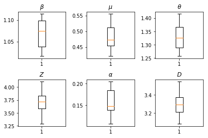
نتائج استنتاجاتنا. نحن رسم القيم كحد أقصى احتمال لجميع معلمتين العالمية لإظهار التباين في انحاء لدينا num_batches أشواط مستقلة الاستدلال. هذا يتوافق مع الجدول S1 في المواد التكميلية.
fig, axs = plt.subplots(2, 3)
axs[0, 0].boxplot(best_parameters.documented_infectious_tx_rate,
                  whis=(2.5,97.5), sym='')
axs[0, 0].set_title(r'$\beta$')

axs[0, 1].boxplot(best_parameters.undocumented_infectious_tx_relative_rate,
                  whis=(2.5,97.5), sym='')
axs[0, 1].set_title(r'$\mu$')

axs[0, 2].boxplot(best_parameters.intercity_underreporting_factor,
                  whis=(2.5,97.5), sym='')
axs[0, 2].set_title(r'$\theta$')

axs[1, 0].boxplot(best_parameters.average_latency_period,
                  whis=(2.5,97.5), sym='')
axs[1, 0].set_title(r'$Z$')

axs[1, 1].boxplot(best_parameters.fraction_of_documented_infections,
                  whis=(2.5,97.5), sym='')
axs[1, 1].set_title(r'$\alpha$')

axs[1, 2].boxplot(best_parameters.average_infection_duration,
                  whis=(2.5,97.5), sym='')
axs[1, 2].set_title(r'$D$')
plt.tight_layout()