| | |  GitHub-এ উৎস দেখুন GitHub-এ উৎস দেখুন | |
এটি লি এট আল-এর 16 মার্চ 2020 কাগজের টেনসরফ্লো সম্ভাব্যতা পোর্ট। আমরা বিশ্বস্ততার সাথে টেনসরফ্লো সম্ভাব্যতা প্ল্যাটফর্মে মূল লেখকের পদ্ধতি এবং ফলাফলগুলি পুনরুত্পাদন করি, আধুনিক মহামারীবিদ্যা মডেলিংয়ের সেটিংয়ে TFP-এর কিছু ক্ষমতা প্রদর্শন করে। TensorFlow-এ পোর্ট করা আমাদের মূল ম্যাটল্যাব কোডের সাপেক্ষে ~10x স্পিডআপ দেয়, এবং যেহেতু TensorFlow সম্ভাব্যতা ব্যাপকভাবে ভেক্টরাইজড ব্যাচ কম্পিউটেশনকে সমর্থন করে, এছাড়াও শত শত স্বাধীন প্রতিলিপিতে সুবিধাজনকভাবে স্কেল করে।
আসল কাগজ
রুইয়ুন লি, সেন পেই, বিন চেন, ইমেং সং, তাও ঝাং, ওয়ান ইয়াং এবং জেফরি শামান। উল্লেখযোগ্য নথিভুক্ত সংক্রমণ নভেল করোনাভাইরাস (SARS-CoV2) এর দ্রুত বিস্তারকে সহজতর করে। (2020), ডোই: https://doi.org/10.1126/science.abb3221 ।
সারাংশ:। "প্রাদুর্ভাব এবং অনথিভুক্ত উপন্যাস coronavirus (Sars-CoV2) সংক্রমণ contagiousness হিসেব সামগ্রিক প্রাদুর্ভাব এবং এই রোগের পৃথিবীব্যাপি সম্ভাব্য বোঝার জন্য গুরুত্বপূর্ণ এখানে আমরা গতিশীলতা ডেটা, একটি সাথে চীন মধ্যে রিপোর্ট সংক্রমণের পর্যবেক্ষণ ব্যবহার করেন, SARS-CoV2 এর সাথে সম্পর্কিত জটিল মহামারী সংক্রান্ত বৈশিষ্ট্যগুলি অনুমান করার জন্য নেটওয়ার্কযুক্ত গতিশীল মেটাপোপুলেশন মডেল এবং বায়েসিয়ান ইনফারেন্স, যার মধ্যে অনথিভুক্ত সংক্রমণের ভগ্নাংশ এবং তাদের সংক্রামকতা রয়েছে। আমরা অনুমান করি যে সমস্ত সংক্রমণের 86% অনথিভুক্ত ছিল (95% CI: [82%–90%] ) 23 জানুয়ারী 2020 এর আগে ভ্রমণ বিধিনিষেধ। ব্যক্তি প্রতি, নথিভুক্ত সংক্রমণের 55% ([46%–62%]) নথিভুক্ত সংক্রমণের হার ছিল, তবুও, তাদের বেশি সংখ্যার কারণে, অনথিভুক্ত সংক্রমণগুলি ছিল 79 জনের সংক্রমণের উত্স নথিভুক্ত মামলার %। এই ফলাফলগুলি SARS-CoV2 এর দ্রুত ভৌগলিক বিস্তারকে ব্যাখ্যা করে এবং এই ভাইরাসের নিয়ন্ত্রণ বিশেষভাবে চ্যালেঞ্জিং হবে বলে নির্দেশ করে।"
GitHub লিঙ্ক কোড এবং তথ্য।
ওভারভিউ
মডেল একটি হল স্বতন্ত্র-বিভাগীয় রোগ মডেল জন্য "সমর্থ", "উদ্ভাসিত" (সংক্রমিত কিন্তু এখনো সংক্রামক না), "সংক্রামক কখনও-নথিভুক্ত", এবং "অবশেষে নথিভুক্ত সংক্রামক" বগি সঙ্গে। দুটি উল্লেখযোগ্য বৈশিষ্ট্য রয়েছে: 375টি চীনা শহরের প্রতিটির জন্য পৃথক বগি, লোকেরা কীভাবে এক শহর থেকে অন্য শহরে ভ্রমণ করে সে সম্পর্কে একটি অনুমান সহ; এবং সংক্রমণ প্রতিবেদন বিলম্ব, যাতে একটি মামলা যে হয়ে "অবশেষে নথিভুক্ত সংক্রামক" দিনে \(t\) একটি সম্ভাব্যতার সূত্রাবলি পরে দিন পর্যন্ত পর্যবেক্ষিত ক্ষেত্রে গন্য দেখা নেই।
মডেলটি অনুমান করে যে কখনও নথিভুক্ত নয় এমন কেসগুলি মৃদু হওয়ার কারণে অনথিভুক্ত হয় এবং এইভাবে কম হারে অন্যদের সংক্রামিত হয়। মূল কাগজে আগ্রহের প্রধান প্যারামিটার হল অপ্রস্তুত মামলার অনুপাত যা বিদ্যমান সংক্রমণের পরিমাণ এবং রোগের বিস্তারের উপর অনথিভুক্ত সংক্রমণের প্রভাব উভয়ই অনুমান করতে।
এই কোল্যাবটি বটম-আপ স্টাইলে কোড ওয়াকথ্রু হিসাবে গঠন করা হয়েছে। ক্রমে, আমরা করব
- ইনজেস্ট করুন এবং সংক্ষিপ্তভাবে ডেটা পরীক্ষা করুন,
- স্টেট স্পেস এবং মডেলের গতিশীলতা সংজ্ঞায়িত করুন,
- Li et al, এবং অনুসরণ করে মডেলে অনুমান করার জন্য ফাংশনের একটি স্যুট তৈরি করুন
- তাদের আহ্বান করুন এবং ফলাফল পরীক্ষা করুন. স্পয়লার: তারা কাগজের মতোই বেরিয়ে আসে।
ইনস্টলেশন এবং পাইথন আমদানি
pip3 install -q tf-nightly tfp-nightly
import collections
import io
import requests
import time
import zipfile

import matplotlib.pyplot as plt
import numpy as np
import pandas as pd

import tensorflow.compat.v2 as tf
import tensorflow_probability as tfp
from tensorflow_probability.python.internal import samplers

tfd = tfp.distributions
tfes = tfp.experimental.sequential
ডেটা আমদানি
আসুন গিথুব থেকে ডেটা আমদানি করি এবং এর কিছু পরিদর্শন করি।
r = requests.get('https://raw.githubusercontent.com/SenPei-CU/COVID-19/master/Data.zip')
z = zipfile.ZipFile(io.BytesIO(r.content))
z.extractall('/tmp/')
raw_incidence = pd.read_csv('/tmp/data/Incidence.csv')
raw_mobility = pd.read_csv('/tmp/data/Mobility.csv')
raw_population = pd.read_csv('/tmp/data/pop.csv')
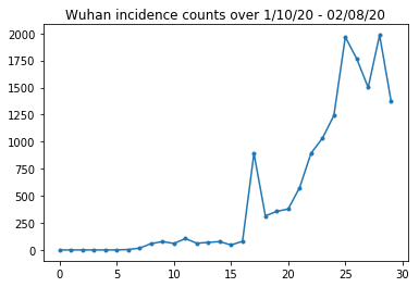
নীচে আমরা প্রতিদিন কাঁচা ঘটনা গণনা দেখতে পারি। আমরা প্রথম 14 দিনে (10 জানুয়ারী থেকে 23শে জানুয়ারী) সবচেয়ে বেশি আগ্রহী, কারণ 23 তারিখে ভ্রমণ নিষেধাজ্ঞাগুলি জারি করা হয়েছিল৷ কাগজটি বিভিন্ন পরামিতি সহ 10-23 জানুয়ারী এবং 23+ জানুয়ারী আলাদাভাবে মডেলিং করে এর সাথে কাজ করে; আমরা শুধু আমাদের প্রজননকে আগের সময়ের মধ্যে সীমাবদ্ধ রাখব।
raw_incidence.drop('Date', axis=1)  # The 'Date' column is all 1/18/21
# Luckily the days are in order, starting on January 10th, 2020.
চলুন উহানের ঘটনা গণনাকে বিবেক-চেক করি।
plt.plot(raw_incidence.Wuhan, '.-')
plt.title('Wuhan incidence counts over 1/10/20 - 02/08/20')
plt.show()
এ পর্যন্ত সব ঠিকই. এখন প্রাথমিক জনসংখ্যা গণনা.
raw_population
আসুন আমরা পরীক্ষা করি এবং রেকর্ড করি কোন এন্ট্রি উহান।
raw_population['City'][169]
'Wuhan'
WUHAN_IDX = 169
এবং এখানে আমরা বিভিন্ন শহরের মধ্যে গতিশীলতা ম্যাট্রিক্স দেখতে পাই। এটি প্রথম 14 দিনে বিভিন্ন শহরের মধ্যে চলাচলকারী লোকের সংখ্যার জন্য একটি প্রক্সি। এটি 2018 লুনার নিউ ইয়ার সিজনের জন্য টেনসেন্টের দেওয়া GPS রেকর্ড থেকে নেওয়া হয়েছে। কিছু অজানা (অনুমান সাপেক্ষে) ধ্রুবক ফ্যাক্টর হিসেবে 2020 সিজনের সময় লি এট মডেল গতিশীলতা \(\theta\) বার করেছেন।
raw_mobility
পরিশেষে, আসুন আমরা এই সবগুলিকে নম্পি অ্যারেতে প্রিপ্রসেস করি যা আমরা গ্রাস করতে পারি।
# The given populations are only "initial" because of intercity mobility during
# the holiday season.
initial_population = raw_population['Population'].to_numpy().astype(np.float32)
গতিশীলতা ডেটাকে একটি [L, L, T]-আকৃতির টেনসরে রূপান্তর করুন, যেখানে L হল অবস্থানের সংখ্যা এবং T হল টাইমস্টেপের সংখ্যা।
daily_mobility_matrices = []
for i in range(1, 15):
  day_mobility = raw_mobility[raw_mobility['Day'] == i]

  # Make a matrix of daily mobilities.
  z = pd.crosstab(
      day_mobility.Origin,
      day_mobility.Destination,
      values=day_mobility['Mobility Index'], aggfunc='sum', dropna=False)

  # Include every city, even if there are no rows for some in the raw data on
  # some day.  This uses the sort order of `raw_population`.
  z = z.reindex(index=raw_population['City'], columns=raw_population['City'],
                fill_value=0)
  # Finally, fill any missing entries with 0. This means no mobility.
  z = z.fillna(0)
  daily_mobility_matrices.append(z.to_numpy())

mobility_matrix_over_time = np.stack(daily_mobility_matrices, axis=-1).astype(
    np.float32)
অবশেষে পর্যবেক্ষণ করা সংক্রমণ নিন এবং একটি [L, T] টেবিল তৈরি করুন।
# Remove the date parameter and take the first 14 days.
observed_daily_infectious_count = raw_incidence.to_numpy()[:14, 1:]
observed_daily_infectious_count = np.transpose(
    observed_daily_infectious_count).astype(np.float32)
এবং ডবল-চেক করুন যে আমরা যেভাবে চেয়েছিলাম সেভাবে আকারগুলি পেয়েছি। একটি অনুস্মারক হিসাবে, আমরা 375টি শহর এবং 14 দিন কাজ করছি৷
print('Mobility Matrix over time should have shape (375, 375, 14): {}'.format(
    mobility_matrix_over_time.shape))
print('Observed Infectious should have shape (375, 14): {}'.format(
    observed_daily_infectious_count.shape))
print('Initial population should have shape (375): {}'.format(
    initial_population.shape))
Mobility Matrix over time should have shape (375, 375, 14): (375, 375, 14)
Observed Infectious should have shape (375, 14): (375, 14)
Initial population should have shape (375): (375,)
স্টেট এবং প্যারামিটার সংজ্ঞায়িত করা
আমাদের মডেল সংজ্ঞায়িত শুরু করা যাক. মডেল আমরা প্রতিলিপি করা হয় একটি একটি বৈচিত্র হয় সেয়ীর মডেল । এই ক্ষেত্রে আমাদের নিম্নলিখিত সময়-পরিবর্তিত অবস্থা রয়েছে:
- \(S\): প্রতিটি শহরে রোগ সমর্থ লোকের সংখ্যা।
- \(E\): রোগের উন্মুক্ত প্রতিটি শহরের লোকের সংখ্যা কিন্তু সংক্রামক এখনো। জৈবিকভাবে, এটি রোগের সংক্রামনের সাথে মিলে যায়, যার ফলে সমস্ত উন্মুক্ত ব্যক্তিরা শেষ পর্যন্ত সংক্রামক হয়ে ওঠে।
- \(I^u\): প্রতিটি শহর যারা সংক্রামক কিন্তু অনথিভুক্ত মানুষের সংখ্যা। মডেলে, এর আসলে মানে "কখনও নথিভুক্ত করা হবে না"।
- \(I^r\): প্রতিটি শহর যারা সংক্রামক এবং যেমন নথিভুক্ত হয় মানুষের সংখ্যা। লি এট মডেল প্রতিবেদনের বিলম্ব, তাই \(I^r\) আসলে ভালো কিছু অনুরূপ "কেস তীব্র যথেষ্ট ভবিষ্যতে কিছু সময়ে নথিভুক্ত করা হয়"।
আমরা নীচের হিসাবে দেখব, আমরা সময়ের সাথে সাথে একটি এনসেম্বল-অ্যাডজাস্টেড কালম্যান ফিল্টার (ইএকেএফ) চালিয়ে এই রাজ্যগুলির অনুমান করব৷ EAKF-এর রাজ্য ভেক্টর হল এই প্রতিটি পরিমাণের জন্য একটি শহর-সূচীযুক্ত ভেক্টর।
মডেলটিতে নিম্নলিখিত অনুমানযোগ্য বৈশ্বিক, সময়-অপরিবর্তনীয় পরামিতি রয়েছে:
- \(\beta\): নথিভুক্ত-সংক্রামক ব্যক্তি কারণে সংক্রমণ হার।
- \(\mu\): অনথিভুক্ত-সংক্রামক ব্যক্তি কারণে আপেক্ষিক সংক্রমণ হার। এই পণ্য মাধ্যমে কাজ করবে \(\mu \beta\)।
- \(\theta\): আন্তনগর গতিশীলতা ফ্যাক্টর। এটি গতিশীলতা ডেটার আন্ডার রিপোর্টিং (এবং 2018 থেকে 2020 পর্যন্ত জনসংখ্যা বৃদ্ধির জন্য) সংশোধন করার জন্য 1টির চেয়ে বেশি একটি ফ্যাক্টর।
- \(Z\): গড় ডিম ফুটতে (অর্থাত, "উদ্ভাসিত" রাজ্যের সময়)।
- \(\alpha\)(অবশেষে) নথিভুক্ত এই সংক্রমণ তীব্র যথেষ্ট হতে ভগ্নাংশ হল:।
- \(D\): সংক্রমণ গড় সময়কাল (অর্থাত, হয় "সংক্রামক" রাজ্যের সময়)।
আমরা রাজ্যগুলির জন্য EAKF এর চারপাশে একটি পুনরাবৃত্তিমূলক-ফিল্টারিং লুপ সহ এই পরামিতিগুলির জন্য বিন্দু অনুমান নির্ণয় করব।
মডেলটি অ-অনুমানিত ধ্রুবকের উপরও নির্ভর করে:
- \(M\): আন্তনগর গতিশীলতা ম্যাট্রিক্স। এটি সময়-পরিবর্তনশীল এবং প্রদত্ত অনুমান। রিকল এটি অনুমিত পরামিতি দ্বারা স্কেল করা হচ্ছে \(\theta\) শহরগুলির মধ্যে প্রকৃত জনসংখ্যা আন্দোলন দিতে।
- \(N\): প্রতিটি শহরে মানুষ মোট সংখ্যা। প্রাথমিক জনগোষ্ঠী নেয়া হয় হিসেবে দেওয়া, এবং জনসংখ্যার সময় প্রকরণ গতিশীলতা নম্বর থেকে নির্ণয় করা হয় \(\theta M\)।
প্রথমত, আমরা আমাদের স্টেট এবং প্যারামিটার ধরে রাখার জন্য নিজেদের কিছু ডেটা স্ট্রাকচার দিই।
SEIRComponents = collections.namedtuple(
  typename='SEIRComponents',
  field_names=[
    'susceptible',              # S
    'exposed',                  # E
    'documented_infectious',    # I^r
    'undocumented_infectious',  # I^u
    # This is the count of new cases in the "documented infectious" compartment.
    # We need this because we will introduce a reporting delay, between a person
    # entering I^r and showing up in the observable case count data.
    # This can't be computed from the cumulative `documented_infectious` count,
    # because some portion of that population will move to the 'recovered'
    # state, which we aren't tracking explicitly.
    'daily_new_documented_infectious'])

ModelParams = collections.namedtuple(
    typename='ModelParams',
    field_names=[
      'documented_infectious_tx_rate',             # Beta
      'undocumented_infectious_tx_relative_rate',  # Mu
      'intercity_underreporting_factor',           # Theta
      'average_latency_period',                    # Z
      'fraction_of_documented_infections',         # Alpha
      'average_infection_duration'                 # D
    ]
)
আমরা প্যারামিটারের মানগুলির জন্য Li et al এর সীমানাও কোড করি।
PARAMETER_LOWER_BOUNDS = ModelParams(
    documented_infectious_tx_rate=0.8,
    undocumented_infectious_tx_relative_rate=0.2,
    intercity_underreporting_factor=1.,
    average_latency_period=2.,
    fraction_of_documented_infections=0.02,
    average_infection_duration=2.
)

PARAMETER_UPPER_BOUNDS = ModelParams(
    documented_infectious_tx_rate=1.5,
    undocumented_infectious_tx_relative_rate=1.,
    intercity_underreporting_factor=1.75,
    average_latency_period=5.,
    fraction_of_documented_infections=1.,
    average_infection_duration=5.
)
SEIR ডায়নামিক্স
এখানে আমরা পরামিতি এবং রাষ্ট্রের মধ্যে সম্পর্ক সংজ্ঞায়িত করি।
Li et al (পরিপূরক উপাদান, eqns 1-5) থেকে সময়-গতিবিদ্যার সমীকরণগুলি নিম্নরূপ:
\(\frac{dS_i}{dt} = -\beta \frac{S_i I_i^r}{N_i} - \mu \beta \frac{S_i I_i^u}{N_i} + \theta \sum_k \frac{M_{ij} S_j}{N_j - I_j^r} - + \theta \sum_k \frac{M_{ji} S_j}{N_i - I_i^r}\)
\(\frac{dE_i}{dt} = \beta \frac{S_i I_i^r}{N_i} + \mu \beta \frac{S_i I_i^u}{N_i} -\frac{E_i}{Z} + \theta \sum_k \frac{M_{ij} E_j}{N_j - I_j^r} - + \theta \sum_k \frac{M_{ji} E_j}{N_i - I_i^r}\)
\(\frac{dI^r_i}{dt} = \alpha \frac{E_i}{Z} - \frac{I_i^r}{D}\)
\(\frac{dI^u_i}{dt} = (1 - \alpha) \frac{E_i}{Z} - \frac{I_i^u}{D} + \theta \sum_k \frac{M_{ij} I_j^u}{N_j - I_j^r} - + \theta \sum_k \frac{M_{ji} I^u_j}{N_i - I_i^r}\)
\(N_i = N_i + \theta \sum_j M_{ij} - \theta \sum_j M_{ji}\)
একটি অনুস্মারক হিসেবে \(i\) এবং \(j\) সাবস্ক্রিপ্টগুলোর সূচক শহর। এই সমীকরণগুলি রোগের সময়-বিবর্তনকে মডেল করে
- সংক্রামক ব্যক্তিদের সাথে যোগাযোগ যা আরও সংক্রমণের দিকে পরিচালিত করে;
- "উন্মুক্ত" থেকে "সংক্রামক" অবস্থার একটিতে রোগের অগ্রগতি;
- "সংক্রামক" অবস্থা থেকে পুনরুদ্ধারের দিকে রোগের অগ্রগতি, যা আমরা মডেল করা জনসংখ্যা থেকে অপসারণের মাধ্যমে মডেল করি;
- আন্তঃনগর গতিশীলতা, উন্মুক্ত বা নথিভুক্ত-সংক্রামক ব্যক্তি সহ; এবং
- আন্তঃনগর গতিশীলতার মাধ্যমে দৈনিক শহরের জনসংখ্যার সময়ের পরিবর্তন।
লি এট আলকে অনুসরণ করে, আমরা ধরে নিই যে যাদের কেসগুলি শেষ পর্যন্ত রিপোর্ট করার মতো যথেষ্ট গুরুতর তারা শহরগুলির মধ্যে ভ্রমণ করে না।
এছাড়াও Li et al অনুসরণ করে, আমরা এই গতিবিদ্যাকে শব্দভিত্তিক পয়সন শব্দের বিষয় হিসাবে বিবেচনা করি, অর্থাৎ, প্রতিটি শব্দ আসলে একটি পয়সনের হার, একটি নমুনা যা থেকে প্রকৃত পরিবর্তন পাওয়া যায়। পয়সন শব্দটি শব্দগত কারণ বিয়োগ (যোগ করার বিপরীতে) পয়সন নমুনাগুলি পয়সন-বিতরণ করা ফলাফল দেয় না।
আমরা ক্লাসিক চতুর্থ-ক্রম Runge-Kutta ইন্টিগ্রেটরের সাথে সময়ের সাথে সাথে এই গতিশীলতাগুলিকে বিকশিত করব, তবে প্রথমে আসুন সেই ফাংশনটি সংজ্ঞায়িত করি যা তাদের গণনা করে (পয়সন শব্দের নমুনা নেওয়া সহ)।
def sample_state_deltas(
    state, population, mobility_matrix, params, seed, is_deterministic=False):
  """Computes one-step change in state, including Poisson sampling.

  Note that this is coded to support vectorized evaluation on arbitrary-shape
  batches of states.  This is useful, for example, for running multiple
  independent replicas of this model to compute credible intervals for the
  parameters.  We refer to the arbitrary batch shape with the conventional
  `B` in the parameter documentation below.  This function also, of course,
  supports broadcasting over the batch shape.

  Args:
    state: A `SEIRComponents` tuple with fields Tensors of shape
      B + [num_locations] giving the current disease state.
    population: A Tensor of shape B + [num_locations] giving the current city
      populations.
    mobility_matrix: A Tensor of shape B + [num_locations, num_locations] giving
      the current baseline inter-city mobility.
    params: A `ModelParams` tuple with fields Tensors of shape B giving the
      global parameters for the current EAKF run.
    seed: Initial entropy for pseudo-random number generation.  The Poisson
      sampling is repeatable by supplying the same seed.
    is_deterministic: A `bool` flag to turn off Poisson sampling if desired.

  Returns:
    delta: A `SEIRComponents` tuple with fields Tensors of shape
      B + [num_locations] giving the one-day changes in the state, according
      to equations 1-4 above (including Poisson noise per Li et al).
  """
  undocumented_infectious_fraction = state.undocumented_infectious / population
  documented_infectious_fraction = state.documented_infectious / population

  # Anyone not documented as infectious is considered mobile
  mobile_population = (population - state.documented_infectious)
  def compute_outflow(compartment_population):
    raw_mobility = tf.linalg.matvec(
        mobility_matrix, compartment_population / mobile_population)
    return params.intercity_underreporting_factor * raw_mobility
  def compute_inflow(compartment_population):
    raw_mobility = tf.linalg.matmul(
        mobility_matrix,
        (compartment_population / mobile_population)[..., tf.newaxis],
        transpose_a=True)
    return params.intercity_underreporting_factor * tf.squeeze(
        raw_mobility, axis=-1)

  # Helper for sampling the Poisson-variate terms.
  seeds = samplers.split_seed(seed, n=11)
  if is_deterministic:
    def sample_poisson(rate):
      return rate
  else:
    def sample_poisson(rate):
      return tfd.Poisson(rate=rate).sample(seed=seeds.pop())

  # Below are the various terms called U1-U12 in the paper. We combined the
  # first two, which should be fine; both are poisson so their sum is too, and
  # there's no risk (as there could be in other terms) of going negative.
  susceptible_becoming_exposed = sample_poisson(
      state.susceptible *
      (params.documented_infectious_tx_rate *
       documented_infectious_fraction +
       (params.undocumented_infectious_tx_relative_rate *
        params.documented_infectious_tx_rate) *
       undocumented_infectious_fraction))  # U1 + U2

  susceptible_population_inflow = sample_poisson(
      compute_inflow(state.susceptible))  # U3
  susceptible_population_outflow = sample_poisson(
      compute_outflow(state.susceptible))  # U4

  exposed_becoming_documented_infectious = sample_poisson(
      params.fraction_of_documented_infections *
      state.exposed / params.average_latency_period)  # U5
  exposed_becoming_undocumented_infectious = sample_poisson(
      (1 - params.fraction_of_documented_infections) *
      state.exposed / params.average_latency_period)  # U6

  exposed_population_inflow = sample_poisson(
      compute_inflow(state.exposed))  # U7
  exposed_population_outflow = sample_poisson(
      compute_outflow(state.exposed))  # U8

  documented_infectious_becoming_recovered = sample_poisson(
      state.documented_infectious /
      params.average_infection_duration)  # U9
  undocumented_infectious_becoming_recovered = sample_poisson(
      state.undocumented_infectious /
      params.average_infection_duration)  # U10

  undocumented_infectious_population_inflow = sample_poisson(
      compute_inflow(state.undocumented_infectious))  # U11
  undocumented_infectious_population_outflow = sample_poisson(
      compute_outflow(state.undocumented_infectious))  # U12

  # The final state_deltas
  return SEIRComponents(
      # Equation [1]
      susceptible=(-susceptible_becoming_exposed +
                   susceptible_population_inflow +
                   -susceptible_population_outflow),
      # Equation [2]
      exposed=(susceptible_becoming_exposed +
               -exposed_becoming_documented_infectious +
               -exposed_becoming_undocumented_infectious +
               exposed_population_inflow +
               -exposed_population_outflow),
      # Equation [3]
      documented_infectious=(
          exposed_becoming_documented_infectious +
          -documented_infectious_becoming_recovered),
      # Equation [4]
      undocumented_infectious=(
          exposed_becoming_undocumented_infectious +
          -undocumented_infectious_becoming_recovered +
          undocumented_infectious_population_inflow +
          -undocumented_infectious_population_outflow),
      # New to-be-documented infectious cases, subject to the delayed
      # observation model.
      daily_new_documented_infectious=exposed_becoming_documented_infectious)
এখানে ইন্টিগ্রেটর. এই মাধ্যমে PRNG বীজ ক্ষণস্থায়ী ছাড়া সম্পূর্ণরূপে মান, sample_state_deltas যে জন্য Runge-Kutta পদ্ধতি কল আংশিক ধাপের প্রতিটি স্বাধীন পইসন গোলমাল পেতে কাজ করে।
@tf.function(autograph=False)
def rk4_one_step(state, population, mobility_matrix, params, seed):
  """Implement one step of RK4, wrapped around a call to sample_state_deltas."""
  # One seed for each RK sub-step
  seeds = samplers.split_seed(seed, n=4)

  deltas = tf.nest.map_structure(tf.zeros_like, state)
  combined_deltas = tf.nest.map_structure(tf.zeros_like, state)

  for a, b in zip([1., 2, 2, 1.], [6., 3., 3., 6.]):
    next_input = tf.nest.map_structure(
        lambda x, delta, a=a: x + delta / a, state, deltas)
    deltas = sample_state_deltas(
        next_input,
        population,
        mobility_matrix,
        params,
        seed=seeds.pop(), is_deterministic=False)
    combined_deltas = tf.nest.map_structure(
        lambda x, delta, b=b: x + delta / b, combined_deltas, deltas)

  return tf.nest.map_structure(
      lambda s, delta: s + tf.round(delta),
      state, combined_deltas)
আরম্ভ
এখানে আমরা কাগজ থেকে শুরু করার স্কিম বাস্তবায়ন করি।
Li et al অনুসরণ করে, আমাদের অনুমান স্কিম হবে একটি ensemble সমন্বয় Kalman ফিল্টার অভ্যন্তরীণ লুপ, একটি পুনরাবৃত্তি ফিল্টারিং বাইরের লুপ (IF-EAKF) দ্বারা বেষ্টিত। গণনাগতভাবে, এর মানে আমাদের তিন ধরণের আরম্ভের প্রয়োজন:
- অভ্যন্তরীণ EAKF-এর জন্য প্রাথমিক অবস্থা
- বাইরের IF-এর জন্য প্রাথমিক পরামিতি, যা প্রথম EAKF-এর প্রাথমিক পরামিতিও
- একটি IF পুনরাবৃত্তি থেকে পরেরটিতে পরামিতি আপডেট করা, যা প্রথমটি ব্যতীত প্রতিটি EAKF-এর প্রাথমিক পরামিতি হিসাবে কাজ করে।
def initialize_state(num_particles, num_batches, seed):
  """Initialize the state for a batch of EAKF runs.

  Args:
    num_particles: `int` giving the number of particles for the EAKF.
    num_batches: `int` giving the number of independent EAKF runs to
      initialize in a vectorized batch.
    seed: PRNG entropy.

  Returns:
    state: A `SEIRComponents` tuple with Tensors of shape [num_particles,
      num_batches, num_cities] giving the initial conditions in each
      city, in each filter particle, in each batch member.
  """
  num_cities = mobility_matrix_over_time.shape[-2]
  state_shape = [num_particles, num_batches, num_cities]
  susceptible = initial_population * np.ones(state_shape, dtype=np.float32)
  documented_infectious = np.zeros(state_shape, dtype=np.float32)
  daily_new_documented_infectious = np.zeros(state_shape, dtype=np.float32)

  # Following Li et al, initialize Wuhan with up to 2000 people exposed
  # and another up to 2000 undocumented infectious.
  rng = np.random.RandomState(seed[0] % (2**31 - 1))
  wuhan_exposed = rng.randint(
      0, 2001, [num_particles, num_batches]).astype(np.float32)
  wuhan_undocumented_infectious = rng.randint(
      0, 2001, [num_particles, num_batches]).astype(np.float32)

  # Also following Li et al, initialize cities adjacent to Wuhan with three
  # days' worth of additional exposed and undocumented-infectious cases,
  # as they may have traveled there before the beginning of the modeling
  # period.
  exposed = 3 * mobility_matrix_over_time[
      WUHAN_IDX, :, 0] * wuhan_exposed[
          ..., np.newaxis] / initial_population[WUHAN_IDX]
  undocumented_infectious = 3 * mobility_matrix_over_time[
      WUHAN_IDX, :, 0] * wuhan_undocumented_infectious[
          ..., np.newaxis] / initial_population[WUHAN_IDX]

  exposed[..., WUHAN_IDX] = wuhan_exposed
  undocumented_infectious[..., WUHAN_IDX] = wuhan_undocumented_infectious

  # Following Li et al, we do not remove the inital exposed and infectious
  # persons from the susceptible population.
  return SEIRComponents(
      susceptible=tf.constant(susceptible),
      exposed=tf.constant(exposed),
      documented_infectious=tf.constant(documented_infectious),
      undocumented_infectious=tf.constant(undocumented_infectious),
      daily_new_documented_infectious=tf.constant(daily_new_documented_infectious))

def initialize_params(num_particles, num_batches, seed):
  """Initialize the global parameters for the entire inference run.

  Args:
    num_particles: `int` giving the number of particles for the EAKF.
    num_batches: `int` giving the number of independent EAKF runs to
      initialize in a vectorized batch.
    seed: PRNG entropy.

  Returns:
    params: A `ModelParams` tuple with fields Tensors of shape
      [num_particles, num_batches] giving the global parameters
      to use for the first batch of EAKF runs.
  """
  # We have 6 parameters. We'll initialize with a Sobol sequence,
  # covering the hyper-rectangle defined by our parameter limits.
  halton_sequence = tfp.mcmc.sample_halton_sequence(
      dim=6, num_results=num_particles * num_batches, seed=seed)
  halton_sequence = tf.reshape(
      halton_sequence, [num_particles, num_batches, 6])
  halton_sequences = tf.nest.pack_sequence_as(
      PARAMETER_LOWER_BOUNDS, tf.split(
          halton_sequence, num_or_size_splits=6, axis=-1))
  def interpolate(minval, maxval, h):
    return (maxval - minval) * h + minval
  return tf.nest.map_structure(
      interpolate,
      PARAMETER_LOWER_BOUNDS, PARAMETER_UPPER_BOUNDS, halton_sequences)

def update_params(num_particles, num_batches,
                  prev_params, parameter_variance, seed):
  """Update the global parameters between EAKF runs.

  Args:
    num_particles: `int` giving the number of particles for the EAKF.
    num_batches: `int` giving the number of independent EAKF runs to
      initialize in a vectorized batch.
    prev_params: A `ModelParams` tuple of the parameters used for the previous
      EAKF run.
    parameter_variance: A `ModelParams` tuple specifying how much to drift
      each parameter.
    seed: PRNG entropy.

  Returns:
    params: A `ModelParams` tuple with fields Tensors of shape
      [num_particles, num_batches] giving the global parameters
      to use for the next batch of EAKF runs.
  """
  # Initialize near the previous set of parameters. This is the first step
  # in Iterated Filtering.
  seeds = tf.nest.pack_sequence_as(
      prev_params, samplers.split_seed(seed, n=len(prev_params)))
  return tf.nest.map_structure(
      lambda x, v, seed: x + tf.math.sqrt(v) * tf.random.stateless_normal([
          num_particles, num_batches, 1], seed=seed),
      prev_params, parameter_variance, seeds)
বিলম্ব
এই মডেলের গুরুত্বপূর্ণ বৈশিষ্ট্যগুলির মধ্যে একটি হল এই বিষয়টির সুস্পষ্ট হিসাব গ্রহণ করা যে সংক্রমণগুলি শুরু হওয়ার চেয়ে পরে রিপোর্ট করা হয়। অর্থাৎ আমরা আশা যে একজন ব্যক্তি যিনি থেকে চলে আসে \(E\) করার কুঠরি \(I^r\) দিনে কুঠরি \(t\) না কিছু পরে দিন পর্যন্ত পর্যবেক্ষণযোগ্য রিপোর্ট ক্ষেত্রে গন্য মধ্যে প্রদর্শিত হতে পারে।
আমরা অনুমান করি যে বিলম্বটি গামা-বিতরণ করা হয়েছে। Li et al অনুসরণ করে, আমরা আকৃতির জন্য 1.85 ব্যবহার করি এবং 9 দিনের গড় রিপোর্টিং বিলম্ব তৈরি করতে হারকে প্যারামিটারাইজ করি।
def raw_reporting_delay_distribution(gamma_shape=1.85, reporting_delay=9.):
  return tfp.distributions.Gamma(
      concentration=gamma_shape, rate=gamma_shape / reporting_delay)
আমাদের পর্যবেক্ষণগুলি বিচ্ছিন্ন, তাই আমরা নিকটতম দিন পর্যন্ত অপরিশোধিত (অবিচ্ছিন্ন) বিলম্বগুলিকে রাউন্ড করব৷ আমাদের কাছে একটি সীমিত ডেটা দিগন্তও রয়েছে, তাই একজন একক ব্যক্তির জন্য বিলম্ব বিতরণ বাকী দিনগুলিতে একটি শ্রেণীবদ্ধ। সুতরাং আমরা স্যাম্পলিং চেয়ে আরো দক্ষতার সঙ্গে প্রতি-শহর পূর্বাভাস পর্যবেক্ষণ গনা করতে \(O(I^r)\) পরিবর্তে gammas, প্রাক কম্পিউটিং MULTINOMIAL বিলম্ব সম্ভাব্যতা দ্বারা।
def reporting_delay_probs(num_timesteps, gamma_shape=1.85, reporting_delay=9.):
  gamma_dist = raw_reporting_delay_distribution(gamma_shape, reporting_delay)
  multinomial_probs = [gamma_dist.cdf(1.)]
  for k in range(2, num_timesteps + 1):
    multinomial_probs.append(gamma_dist.cdf(k) - gamma_dist.cdf(k - 1))
  # For samples that are larger than T.
  multinomial_probs.append(gamma_dist.survival_function(num_timesteps))
  multinomial_probs = tf.stack(multinomial_probs)
  return multinomial_probs
নতুন দৈনিক নথিভুক্ত সংক্রামক গণনাগুলিতে এই বিলম্বগুলি বাস্তবে প্রয়োগ করার কোড এখানে রয়েছে:
def delay_reporting(
    daily_new_documented_infectious, num_timesteps, t, multinomial_probs, seed):
  # This is the distribution of observed infectious counts from the current
  # timestep.

  raw_delays = tfd.Multinomial(
      total_count=daily_new_documented_infectious,
      probs=multinomial_probs).sample(seed=seed)

  # The last bucket is used for samples that are out of range of T + 1. Thus
  # they are not going to be observable in this model.
  clipped_delays = raw_delays[..., :-1]

  # We can also remove counts that are such that t + i >= T.
  clipped_delays = clipped_delays[..., :num_timesteps - t]
  # We finally shift everything by t. That means prepending with zeros.
  return tf.concat([
      tf.zeros(
          tf.concat([
              tf.shape(clipped_delays)[:-1], [t]], axis=0),
          dtype=clipped_delays.dtype),
      clipped_delays], axis=-1)
অনুমান
প্রথমে আমরা অনুমানের জন্য কিছু ডেটা স্ট্রাকচার সংজ্ঞায়িত করব।
বিশেষ করে, আমরা ইটারেটেড ফিল্টারিং করতে চাই, যা অনুমান করার সময় স্টেট এবং প্যারামিটার একসাথে প্যাকেজ করে। সুতরাং আমরা একটি সংজ্ঞায়িত করব ParameterStatePair অবজেক্ট।
আমরা মডেলের যেকোনো পার্শ্ব তথ্য প্যাকেজ করতে চাই।
ParameterStatePair = collections.namedtuple(
    'ParameterStatePair', ['state', 'params'])

# Info that is tracked and mutated but should not have inference performed over.
SideInfo = collections.namedtuple(
    'SideInfo', [
        # Observations at every time step.
        'observations_over_time',
        'initial_population',
        'mobility_matrix_over_time',
        'population',
        # Used for variance of measured observations.
        'actual_reported_cases',
        # Pre-computed buckets for the multinomial distribution.
        'multinomial_probs',
        'seed',
    ])

# Cities can not fall below this fraction of people
MINIMUM_CITY_FRACTION = 0.6

# How much to inflate the covariance by.
INFLATION_FACTOR = 1.1

INFLATE_FN = tfes.inflate_by_scaled_identity_fn(INFLATION_FACTOR)
এখানে এনসেম্বল কালম্যান ফিল্টারের জন্য প্যাকেজ করা সম্পূর্ণ পর্যবেক্ষণ মডেল।
আকর্ষণীয় বৈশিষ্ট্য হল রিপোর্টিং বিলম্ব (আগের হিসাবে গণনা)। মূল প্রজেক্টের মডেল নির্গত daily_new_documented_infectious প্রতিটি সময় পদে পদে প্রতিটি শহরের জন্য।
# We observe the observed infections.
def observation_fn(t, state_params, extra):
  """Generate reported cases.

  Args:
    state_params: A `ParameterStatePair` giving the current parameters
      and state.
    t: Integer giving the current time.
    extra: A `SideInfo` carrying auxiliary information.

  Returns:
    observations: A Tensor of predicted observables, namely new cases
      per city at time `t`.
    extra: Update `SideInfo`.
  """
  # Undo padding introduced in `inference`.
  daily_new_documented_infectious = state_params.state.daily_new_documented_infectious[..., 0]
  # Number of people that we have already committed to become
  # observed infectious over time.
  # shape: batch + [num_particles, num_cities, time]
  observations_over_time = extra.observations_over_time
  num_timesteps = observations_over_time.shape[-1]

  seed, new_seed = samplers.split_seed(extra.seed, salt='reporting delay')

  daily_delayed_counts = delay_reporting(
      daily_new_documented_infectious, num_timesteps, t,
      extra.multinomial_probs, seed)
  observations_over_time = observations_over_time + daily_delayed_counts

  extra = extra._replace(
      observations_over_time=observations_over_time,
      seed=new_seed)

  # Actual predicted new cases, re-padded.
  adjusted_observations = observations_over_time[..., t][..., tf.newaxis]
  # Finally observations have variance that is a function of the true observations:
  return tfd.MultivariateNormalDiag(
      loc=adjusted_observations,
      scale_diag=tf.math.maximum(
          2., extra.actual_reported_cases[..., t][..., tf.newaxis] / 2.)), extra
এখানে আমরা রূপান্তর গতিবিদ্যা সংজ্ঞায়িত. আমরা ইতিমধ্যে শব্দার্থিক কাজ করেছি; এখানে আমরা এটিকে শুধুমাত্র EAKF ফ্রেমওয়ার্কের জন্য প্যাকেজ করি এবং, Li et al অনুসরণ করে, শহরের জনসংখ্যাকে খুব ছোট হওয়া থেকে রোধ করতে ক্লিপ করি।
def transition_fn(t, state_params, extra):
  """SEIR dynamics.

  Args:
    state_params: A `ParameterStatePair` giving the current parameters
      and state.
    t: Integer giving the current time.
    extra: A `SideInfo` carrying auxiliary information.

  Returns:
    state_params: A `ParameterStatePair` predicted for the next time step.
    extra: Updated `SideInfo`.
  """
  mobility_t = extra.mobility_matrix_over_time[..., t]
  new_seed, rk4_seed = samplers.split_seed(extra.seed, salt='Transition')
  new_state = rk4_one_step(
      state_params.state,
      extra.population,
      mobility_t,
      state_params.params,
      seed=rk4_seed)

  # Make sure population doesn't go below MINIMUM_CITY_FRACTION.
  new_population = (
      extra.population + state_params.params.intercity_underreporting_factor * (
          # Inflow
          tf.reduce_sum(mobility_t, axis=-2) -
          # Outflow
          tf.reduce_sum(mobility_t, axis=-1)))
  new_population = tf.where(
      new_population < MINIMUM_CITY_FRACTION * extra.initial_population,
      extra.initial_population * MINIMUM_CITY_FRACTION,
      new_population)

  extra = extra._replace(population=new_population, seed=new_seed)

  # The Ensemble Kalman Filter code expects the transition function to return a distribution.
  # As the dynamics and noise are encapsulated above, we construct a `JointDistribution` that when
  # sampled, returns the values above.

  new_state = tfd.JointDistributionNamed(
      model=tf.nest.map_structure(lambda x: tfd.VectorDeterministic(x), new_state))
  params = tfd.JointDistributionNamed(
      model=tf.nest.map_structure(lambda x: tfd.VectorDeterministic(x), state_params.params))

  state_params = tfd.JointDistributionNamed(
      model=ParameterStatePair(state=new_state, params=params))

  return state_params, extra
অবশেষে আমরা অনুমান পদ্ধতি সংজ্ঞায়িত করি। এটি দুটি লুপ, বাইরের লুপটি পুনরাবৃত্তি ফিল্টারিং এবং ভিতরের লুপটি হল এনসেম্বল অ্যাডজাস্টমেন্ট কালম্যান ফিল্টারিং।
# Use tf.function to speed up EAKF prediction and updates.
ensemble_kalman_filter_predict = tf.function(
    tfes.ensemble_kalman_filter_predict, autograph=False)
ensemble_adjustment_kalman_filter_update = tf.function(
    tfes.ensemble_adjustment_kalman_filter_update, autograph=False)

def inference(
    num_ensembles,
    num_batches,
    num_iterations,
    actual_reported_cases,
    mobility_matrix_over_time,
    seed=None,
    # This is how much to reduce the variance by in every iterative
    # filtering step.
    variance_shrinkage_factor=0.9,
    # Days before infection is reported.
    reporting_delay=9.,
    # Shape parameter of Gamma distribution.
    gamma_shape_parameter=1.85):
  """Inference for the Shaman, et al. model.

  Args:
    num_ensembles: Number of particles to use for EAKF.
    num_batches: Number of batches of IF-EAKF to run.
    num_iterations: Number of iterations to run iterative filtering.
    actual_reported_cases: `Tensor` of shape `[L, T]` where `L` is the number
      of cities, and `T` is the timesteps.
    mobility_matrix_over_time: `Tensor` of shape `[L, L, T]` which specifies the
      mobility between locations over time.
    variance_shrinkage_factor: Python `float`. How much to reduce the
      variance each iteration of iterated filtering.
    reporting_delay: Python `float`. How many days before the infection
      is reported.
    gamma_shape_parameter: Python `float`. Shape parameter of Gamma distribution
      of reporting delays.

  Returns:
    result: A `ModelParams` with fields Tensors of shape [num_batches],
      containing the inferred parameters at the final iteration.
  """
  print('Starting inference.')
  num_timesteps = actual_reported_cases.shape[-1]
  params_per_iter = []

  multinomial_probs = reporting_delay_probs(
      num_timesteps, gamma_shape_parameter, reporting_delay)

  seed = samplers.sanitize_seed(seed, salt='Inference')

  for i in range(num_iterations):
    start_if_time = time.time()
    seeds = samplers.split_seed(seed, n=4, salt='Initialize')
    if params_per_iter:
      parameter_variance = tf.nest.map_structure(
          lambda minval, maxval: variance_shrinkage_factor ** (
              2 * i) * (maxval - minval) ** 2 / 4.,
          PARAMETER_LOWER_BOUNDS, PARAMETER_UPPER_BOUNDS)
      params_t = update_params(
          num_ensembles,
          num_batches,
          prev_params=params_per_iter[-1],
          parameter_variance=parameter_variance,
          seed=seeds.pop())
    else:
      params_t = initialize_params(num_ensembles, num_batches, seed=seeds.pop())

    state_t = initialize_state(num_ensembles, num_batches, seed=seeds.pop())
    population_t = sum(x for x in state_t)
    observations_over_time = tf.zeros(
        [num_ensembles,
         num_batches,
         actual_reported_cases.shape[0], num_timesteps])

    extra = SideInfo(
        observations_over_time=observations_over_time,
        initial_population=tf.identity(population_t),
        mobility_matrix_over_time=mobility_matrix_over_time,
        population=population_t,
        multinomial_probs=multinomial_probs,
        actual_reported_cases=actual_reported_cases,
        seed=seeds.pop())

    # Clip states
    state_t = clip_state(state_t, population_t)
    params_t = clip_params(params_t, seed=seeds.pop())

    # Accrue the parameter over time. We'll be averaging that
    # and using that as our MLE estimate.
    params_over_time = tf.nest.map_structure(
        lambda x: tf.identity(x), params_t)

    state_params = ParameterStatePair(state=state_t, params=params_t)

    eakf_state = tfes.EnsembleKalmanFilterState(
        step=tf.constant(0), particles=state_params, extra=extra)

    for j in range(num_timesteps):
      seeds = samplers.split_seed(eakf_state.extra.seed, n=3)

      extra = extra._replace(seed=seeds.pop())

      # Predict step.

      # Inflate and clip.
      new_particles = INFLATE_FN(eakf_state.particles)
      state_t = clip_state(new_particles.state, eakf_state.extra.population)
      params_t = clip_params(new_particles.params, seed=seeds.pop())
      eakf_state = eakf_state._replace(
          particles=ParameterStatePair(params=params_t, state=state_t))

      eakf_predict_state = ensemble_kalman_filter_predict(eakf_state, transition_fn)

      # Clip the state and particles.
      state_params = eakf_predict_state.particles
      state_t = clip_state(
          state_params.state, eakf_predict_state.extra.population)
      state_params = ParameterStatePair(state=state_t, params=state_params.params)

      # We preprocess the state and parameters by affixing a 1 dimension. This is because for
      # inference, we treat each city as independent. We could also introduce localization by
      # considering cities that are adjacent.
      state_params = tf.nest.map_structure(lambda x: x[..., tf.newaxis], state_params)
      eakf_predict_state = eakf_predict_state._replace(particles=state_params)

      # Update step.

      eakf_update_state = ensemble_adjustment_kalman_filter_update(
          eakf_predict_state,
          actual_reported_cases[..., j][..., tf.newaxis],
          observation_fn)

      state_params = tf.nest.map_structure(
          lambda x: x[..., 0], eakf_update_state.particles)

      # Clip to ensure parameters / state are well constrained.
      state_t = clip_state(
          state_params.state, eakf_update_state.extra.population)

      # Finally for the parameters, we should reduce over all updates. We get
      # an extra dimension back so let's do that.
      params_t = tf.nest.map_structure(
          lambda x, y: x + tf.reduce_sum(y[..., tf.newaxis] - x, axis=-2, keepdims=True),
          eakf_predict_state.particles.params, state_params.params)
      params_t = clip_params(params_t, seed=seeds.pop())
      params_t = tf.nest.map_structure(lambda x: x[..., 0], params_t)

      state_params = ParameterStatePair(state=state_t, params=params_t)
      eakf_state = eakf_update_state
      eakf_state = eakf_state._replace(particles=state_params)

      # Flatten and collect the inferred parameter at time step t.
      params_over_time = tf.nest.map_structure(
          lambda s, x: tf.concat([s, x], axis=-1), params_over_time, params_t)

    est_params = tf.nest.map_structure(
        # Take the average over the Ensemble and over time.
        lambda x: tf.math.reduce_mean(x, axis=[0, -1])[..., tf.newaxis],
        params_over_time)
    params_per_iter.append(est_params)
    print('Iterated Filtering {} / {} Ran in: {:.2f} seconds'.format(
        i, num_iterations, time.time() - start_if_time))

  return tf.nest.map_structure(
      lambda x: tf.squeeze(x, axis=-1), params_per_iter[-1])
চূড়ান্ত বিশদ: প্যারামিটার এবং স্টেট ক্লিপ করা নিশ্চিত করা হয় যে সেগুলি সীমার মধ্যে রয়েছে এবং অ-নেতিবাচক।
def clip_state(state, population):
  """Clip state to sensible values."""
  state = tf.nest.map_structure(
      lambda x: tf.where(x < 0, 0., x), state)

  # If S > population, then adjust as well.
  susceptible = tf.where(state.susceptible > population, population, state.susceptible)
  return SEIRComponents(
      susceptible=susceptible,
      exposed=state.exposed,
      documented_infectious=state.documented_infectious,
      undocumented_infectious=state.undocumented_infectious,
      daily_new_documented_infectious=state.daily_new_documented_infectious)

def clip_params(params, seed):
  """Clip parameters to bounds."""
  def _clip(p, minval, maxval):
    return tf.where(
        p < minval,
        minval * (1. + 0.1 * tf.random.stateless_uniform(p.shape, seed=seed)),
        tf.where(p > maxval,
                 maxval * (1. - 0.1 * tf.random.stateless_uniform(
                     p.shape, seed=seed)), p))
  params = tf.nest.map_structure(
      _clip, params, PARAMETER_LOWER_BOUNDS, PARAMETER_UPPER_BOUNDS)

  return params
সব একসাথে চালানো
# Let's sample the parameters.
#
# NOTE: Li et al. run inference 1000 times, which would take a few hours.
# Here we run inference 30 times (in a single, vectorized batch).
best_parameters = inference(
    num_ensembles=300,
    num_batches=30,
    num_iterations=10,
    actual_reported_cases=observed_daily_infectious_count,
    mobility_matrix_over_time=mobility_matrix_over_time)
Starting inference.
Iterated Filtering 0 / 10 Ran in: 26.65 seconds
Iterated Filtering 1 / 10 Ran in: 28.69 seconds
Iterated Filtering 2 / 10 Ran in: 28.06 seconds
Iterated Filtering 3 / 10 Ran in: 28.48 seconds
Iterated Filtering 4 / 10 Ran in: 28.57 seconds
Iterated Filtering 5 / 10 Ran in: 28.35 seconds
Iterated Filtering 6 / 10 Ran in: 28.35 seconds
Iterated Filtering 7 / 10 Ran in: 28.19 seconds
Iterated Filtering 8 / 10 Ran in: 28.58 seconds
Iterated Filtering 9 / 10 Ran in: 28.23 seconds
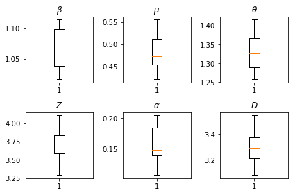
আমাদের অনুমানের ফলাফল। সব বিশ্বব্যাপী paramters আমাদের জুড়ে তাদের প্রকরণ দেখানো হবে তার জন্য আমরা সর্বোচ্চ-সম্ভাবনা মান প্লটে বিভক্ত num_batches অনুমান স্বাধীন রান। এটি সম্পূরক উপকরণগুলিতে টেবিল S1 এর সাথে মিলে যায়।
fig, axs = plt.subplots(2, 3)
axs[0, 0].boxplot(best_parameters.documented_infectious_tx_rate,
                  whis=(2.5,97.5), sym='')
axs[0, 0].set_title(r'$\beta$')

axs[0, 1].boxplot(best_parameters.undocumented_infectious_tx_relative_rate,
                  whis=(2.5,97.5), sym='')
axs[0, 1].set_title(r'$\mu$')

axs[0, 2].boxplot(best_parameters.intercity_underreporting_factor,
                  whis=(2.5,97.5), sym='')
axs[0, 2].set_title(r'$\theta$')

axs[1, 0].boxplot(best_parameters.average_latency_period,
                  whis=(2.5,97.5), sym='')
axs[1, 0].set_title(r'$Z$')

axs[1, 1].boxplot(best_parameters.fraction_of_documented_infections,
                  whis=(2.5,97.5), sym='')
axs[1, 1].set_title(r'$\alpha$')

axs[1, 2].boxplot(best_parameters.average_infection_duration,
                  whis=(2.5,97.5), sym='')
axs[1, 2].set_title(r'$D$')
plt.tight_layout()