| | |  Visualizza la fonte su GitHub Visualizza la fonte su GitHub | |
Questo è un port di TensorFlow Probability dell'omonimo documento del 16 marzo 2020 di Li et al. Riproduciamo fedelmente i metodi e i risultati degli autori originali sulla piattaforma TensorFlow Probability, mostrando alcune delle capacità della TFP nell'ambito della moderna modellazione epidemiologica. Il porting su TensorFlow ci offre un'accelerazione di circa 10 volte rispetto al codice Matlab originale e, poiché TensorFlow Probability supporta in modo pervasivo il calcolo batch vettorizzato, si adatta favorevolmente anche a centinaia di repliche indipendenti.
Carta originale
Ruiyun Li, Sen Pei, Bin Chen, Yimeng Song, Tao Zhang, Wan Yang e Jeffrey Shaman. Un'infezione sostanziale non documentata facilita la rapida diffusione del nuovo coronavirus (SARS-CoV2). (2020), doi: https://doi.org/10.1126/science.abb3221 .
Abstract:. "La stima della prevalenza e contagiosità delle infezioni documentate nuovo coronavirus (SARS-CoV2) è fondamentale per comprendere la prevalenza globale e potenziale pandemia di questa malattia Qui usiamo osservazioni di infezione riportata all'interno della Cina, in combinazione con i dati di mobilità, a modello di metapopolazione dinamica in rete e inferenza bayesiana, per dedurre le caratteristiche epidemiologiche critiche associate a SARS-CoV2, inclusa la frazione di infezioni non documentate e la loro contagiosità.Stimiamo che l'86% di tutte le infezioni non fossero documentate (IC 95%: [82%–90%] ) prima delle restrizioni di viaggio del 23 gennaio 2020. Per persona, il tasso di trasmissione delle infezioni non documentate era del 55% delle infezioni documentate ([46%–62%]), tuttavia, a causa del loro numero maggiore, le infezioni non documentate erano la fonte di infezione per 79 % di casi documentati. Questi risultati spiegano la rapida diffusione geografica di SARS-CoV2 e indicano che il contenimento di questo virus sarà particolarmente impegnativo".
Github collegamento al codice e dati.
Panoramica
Il modello è un modello di malattia compartimentale , con scomparti per "sensibili", "a vista" (infetti ma non ancora contagioso), "non ha mai documentato infettive", e "alla fine documentato infettiva". Ci sono due caratteristiche degne di nota: compartimenti separati per ciascuna delle 375 città cinesi, con un'ipotesi su come le persone viaggiano da una città all'altra; e ritardi nella segnalazione di infezione, in modo che un caso che diventa "fine-documentato infettiva" il giorno \(t\) non si presenta nei casi di conteggi osservati fino a quando un giorno dopo stocastico.
Il modello presuppone che i casi mai documentati finiscano per non essere documentati essendo più miti, e quindi infettino gli altri a un tasso inferiore. Il principale parametro di interesse nel documento originale è la proporzione di casi non documentati, per stimare sia l'estensione dell'infezione esistente, sia l'impatto della trasmissione non documentata sulla diffusione della malattia.
Questa collaborazione è strutturata come una procedura dettagliata del codice in stile bottom-up. In ordine, lo faremo
- Ingerire ed esaminare brevemente i dati,
- Definire lo spazio degli stati e la dinamica del modello,
- Costruisci una suite di funzioni per fare inferenza nel modello che segue Li et al, e
- Invocateli ed esaminate i risultati. Spoiler: escono come la carta.
Installazione e importazioni Python
pip3 install -q tf-nightly tfp-nightly
import collections
import io
import requests
import time
import zipfile

import matplotlib.pyplot as plt
import numpy as np
import pandas as pd

import tensorflow.compat.v2 as tf
import tensorflow_probability as tfp
from tensorflow_probability.python.internal import samplers

tfd = tfp.distributions
tfes = tfp.experimental.sequential
Importazione dati
Importiamo i dati da github e ne ispezioniamo alcuni.
r = requests.get('https://raw.githubusercontent.com/SenPei-CU/COVID-19/master/Data.zip')
z = zipfile.ZipFile(io.BytesIO(r.content))
z.extractall('/tmp/')
raw_incidence = pd.read_csv('/tmp/data/Incidence.csv')
raw_mobility = pd.read_csv('/tmp/data/Mobility.csv')
raw_population = pd.read_csv('/tmp/data/pop.csv')
Di seguito possiamo vedere il conteggio grezzo dell'incidenza al giorno. Siamo più interessati ai primi 14 giorni (dal 10 gennaio al 23 gennaio), poiché le restrizioni di viaggio sono state messe in atto il 23. Il documento si occupa di questo modellando separatamente il 10-23 gennaio e il 23 gennaio+, con parametri diversi; limiteremo semplicemente la nostra riproduzione al periodo precedente.
raw_incidence.drop('Date', axis=1)  # The 'Date' column is all 1/18/21
# Luckily the days are in order, starting on January 10th, 2020.
Controlliamo la sanità mentale che conta l'incidenza di Wuhan.
plt.plot(raw_incidence.Wuhan, '.-')
plt.title('Wuhan incidence counts over 1/10/20 - 02/08/20')
plt.show()
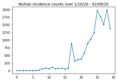
Fin qui tutto bene. Ora conta la popolazione iniziale.
raw_population
Controlliamo e registriamo anche quale voce è Wuhan.
raw_population['City'][169]
'Wuhan'
WUHAN_IDX = 169
E qui vediamo la matrice della mobilità tra le diverse città. Questo è un proxy per il numero di persone che si spostano tra città diverse nei primi 14 giorni. Deriva dai record GPS forniti da Tencent per la stagione del capodanno lunare 2018. Li ed altri mobilità modello durante la stagione 2020, in quanto alcuni sconosciuti (soggetto a deduzione) fattore costante \(\theta\) volte questo.
raw_mobility
Infine, preprocessiamo tutto questo in array numpy che possiamo consumare.
# The given populations are only "initial" because of intercity mobility during
# the holiday season.
initial_population = raw_population['Population'].to_numpy().astype(np.float32)
Converti i dati di mobilità in un tensore a forma di [L, L, T], dove L è il numero di posizioni e T è il numero di fasi temporali.
daily_mobility_matrices = []
for i in range(1, 15):
  day_mobility = raw_mobility[raw_mobility['Day'] == i]

  # Make a matrix of daily mobilities.
  z = pd.crosstab(
      day_mobility.Origin,
      day_mobility.Destination,
      values=day_mobility['Mobility Index'], aggfunc='sum', dropna=False)

  # Include every city, even if there are no rows for some in the raw data on
  # some day.  This uses the sort order of `raw_population`.
  z = z.reindex(index=raw_population['City'], columns=raw_population['City'],
                fill_value=0)
  # Finally, fill any missing entries with 0. This means no mobility.
  z = z.fillna(0)
  daily_mobility_matrices.append(z.to_numpy())

mobility_matrix_over_time = np.stack(daily_mobility_matrices, axis=-1).astype(
    np.float32)
Infine prendi le infezioni osservate e crea una tabella [L, T].
# Remove the date parameter and take the first 14 days.
observed_daily_infectious_count = raw_incidence.to_numpy()[:14, 1:]
observed_daily_infectious_count = np.transpose(
    observed_daily_infectious_count).astype(np.float32)
E ricontrolla che abbiamo ottenuto le forme nel modo desiderato. Come promemoria, stiamo lavorando con 375 città e 14 giorni.
print('Mobility Matrix over time should have shape (375, 375, 14): {}'.format(
    mobility_matrix_over_time.shape))
print('Observed Infectious should have shape (375, 14): {}'.format(
    observed_daily_infectious_count.shape))
print('Initial population should have shape (375): {}'.format(
    initial_population.shape))
Mobility Matrix over time should have shape (375, 375, 14): (375, 375, 14)
Observed Infectious should have shape (375, 14): (375, 14)
Initial population should have shape (375): (375,)
Definizione di stato e parametri
Iniziamo a definire il nostro modello. Il modello che riproduciamo è una variante di un modello di SEIR . In questo caso abbiamo i seguenti stati variabili nel tempo:
- \(S\): Numero di persone sensibili alla malattia in ogni città.
- \(E\): numero di persone in ogni città esposte alla malattia infettiva, ma non ancora. Biologicamente, ciò corrisponde a contrarre la malattia, in quanto tutte le persone esposte alla fine diventano infettive.
- \(I^u\): numero di persone in ogni città che sono infettive, ma non documentato. Nel modello, questo in realtà significa "non sarà mai documentato".
- \(I^r\): numero di persone in ogni città che sono infettive e documentato come tale. Li et al modello di rendicontazione ritardi, così \(I^r\) in realtà corrisponde a qualcosa come "caso è abbastanza grave da essere documentato ad un certo punto in futuro".
Come vedremo di seguito, dedurremo questi stati eseguendo un filtro di Kalman regolato dall'insieme (EAKF) in avanti nel tempo. Il vettore di stato dell'EAKF è un vettore indicizzato per città per ciascuna di queste quantità.
Il modello ha i seguenti parametri globali invariabili nel tempo deducibili:
- \(\beta\): La velocità di trasmissione a causa di individui-infettivi documentati.
- \(\mu\): La velocità di trasmissione relativa dovuta ai singoli irregolari infettivo. Questo agirà attraverso il prodotto \(\mu \beta\).
- \(\theta\): Il fattore di mobilità intercity. Si tratta di un fattore maggiore di 1 che corregge per la sottosegnalazione dei dati sulla mobilità (e per la crescita della popolazione dal 2018 al 2020).
- \(Z\): Il periodo di incubazione medio (vale a dire, il tempo nello stato "esposto").
- \(\alpha\): Questa è la frazione di infezioni basta essere gravi (eventualmente) documentato.
- \(D\): La durata media delle infezioni (cioè, il tempo in uno stato di "infettivo").
Dedurremo le stime puntuali per questi parametri con un ciclo Iterative-Filtering attorno all'EAKF per gli stati.
Il modello dipende anche da costanti non dedotte:
- \(M\): La matrice mobilità interurbani. Questo è variabile nel tempo e si presume dato. Ricordiamo che è scalato dal parametro desunto \(\theta\) per dare i movimenti di popolazione effettiva tra le città.
- \(N\): Il numero totale di persone in ogni città. Le popolazioni iniziali sono presi come dato, e la variazione temporale della popolazione è calcolato dal numero di mobilità \(\theta M\).
Innanzitutto, ci diamo alcune strutture dati per contenere i nostri stati e parametri.
SEIRComponents = collections.namedtuple(
  typename='SEIRComponents',
  field_names=[
    'susceptible',              # S
    'exposed',                  # E
    'documented_infectious',    # I^r
    'undocumented_infectious',  # I^u
    # This is the count of new cases in the "documented infectious" compartment.
    # We need this because we will introduce a reporting delay, between a person
    # entering I^r and showing up in the observable case count data.
    # This can't be computed from the cumulative `documented_infectious` count,
    # because some portion of that population will move to the 'recovered'
    # state, which we aren't tracking explicitly.
    'daily_new_documented_infectious'])

ModelParams = collections.namedtuple(
    typename='ModelParams',
    field_names=[
      'documented_infectious_tx_rate',             # Beta
      'undocumented_infectious_tx_relative_rate',  # Mu
      'intercity_underreporting_factor',           # Theta
      'average_latency_period',                    # Z
      'fraction_of_documented_infections',         # Alpha
      'average_infection_duration'                 # D
    ]
)
Codifichiamo anche i limiti di Li et al per i valori dei parametri.
PARAMETER_LOWER_BOUNDS = ModelParams(
    documented_infectious_tx_rate=0.8,
    undocumented_infectious_tx_relative_rate=0.2,
    intercity_underreporting_factor=1.,
    average_latency_period=2.,
    fraction_of_documented_infections=0.02,
    average_infection_duration=2.
)

PARAMETER_UPPER_BOUNDS = ModelParams(
    documented_infectious_tx_rate=1.5,
    undocumented_infectious_tx_relative_rate=1.,
    intercity_underreporting_factor=1.75,
    average_latency_period=5.,
    fraction_of_documented_infections=1.,
    average_infection_duration=5.
)
SEIR Dynamics
Qui definiamo la relazione tra i parametri e lo stato.
Le equazioni della dinamica del tempo da Li et al (materiale supplementare, eqns 1-5) sono le seguenti:
\(\frac{dS_i}{dt} = -\beta \frac{S_i I_i^r}{N_i} - \mu \beta \frac{S_i I_i^u}{N_i} + \theta \sum_k \frac{M_{ij} S_j}{N_j - I_j^r} - + \theta \sum_k \frac{M_{ji} S_j}{N_i - I_i^r}\)
\(\frac{dE_i}{dt} = \beta \frac{S_i I_i^r}{N_i} + \mu \beta \frac{S_i I_i^u}{N_i} -\frac{E_i}{Z} + \theta \sum_k \frac{M_{ij} E_j}{N_j - I_j^r} - + \theta \sum_k \frac{M_{ji} E_j}{N_i - I_i^r}\)
\(\frac{dI^r_i}{dt} = \alpha \frac{E_i}{Z} - \frac{I_i^r}{D}\)
\(\frac{dI^u_i}{dt} = (1 - \alpha) \frac{E_i}{Z} - \frac{I_i^u}{D} + \theta \sum_k \frac{M_{ij} I_j^u}{N_j - I_j^r} - + \theta \sum_k \frac{M_{ji} I^u_j}{N_i - I_i^r}\)
\(N_i = N_i + \theta \sum_j M_{ij} - \theta \sum_j M_{ji}\)
Come promemoria, il \(i\) e \(j\) città indice indici. Queste equazioni modellano l'evoluzione temporale della malattia attraverso
- Contatto con individui infetti che portano a più infezioni;
- Progressione della malattia da "esposto" a uno degli stati "infettivi";
- Progressione della malattia da stati "infettivi" al recupero, che modelliamo rimuovendo dalla popolazione modellata;
- Mobilità interurbana, comprese le persone esposte o infettive prive di documenti; e
- Variazione temporale delle popolazioni cittadine quotidiane attraverso la mobilità interurbana.
Seguendo Li et al, assumiamo che le persone con casi abbastanza gravi da essere eventualmente denunciati non viaggino tra le città.
Seguendo anche Li et al, trattiamo queste dinamiche come soggette al rumore di Poisson per termini, cioè ogni termine è in realtà la velocità di un Poisson, un campione da cui fornisce il vero cambiamento. Il rumore di Poisson è terminologico perché la sottrazione (anziché l'aggiunta) di campioni di Poisson non produce un risultato con distribuzione di Poisson.
Evolveremo queste dinamiche in avanti nel tempo con il classico integratore Runge-Kutta del quarto ordine, ma prima definiamo la funzione che le calcola (incluso il campionamento del rumore di Poisson).
def sample_state_deltas(
    state, population, mobility_matrix, params, seed, is_deterministic=False):
  """Computes one-step change in state, including Poisson sampling.

  Note that this is coded to support vectorized evaluation on arbitrary-shape
  batches of states.  This is useful, for example, for running multiple
  independent replicas of this model to compute credible intervals for the
  parameters.  We refer to the arbitrary batch shape with the conventional
  `B` in the parameter documentation below.  This function also, of course,
  supports broadcasting over the batch shape.

  Args:
    state: A `SEIRComponents` tuple with fields Tensors of shape
      B + [num_locations] giving the current disease state.
    population: A Tensor of shape B + [num_locations] giving the current city
      populations.
    mobility_matrix: A Tensor of shape B + [num_locations, num_locations] giving
      the current baseline inter-city mobility.
    params: A `ModelParams` tuple with fields Tensors of shape B giving the
      global parameters for the current EAKF run.
    seed: Initial entropy for pseudo-random number generation.  The Poisson
      sampling is repeatable by supplying the same seed.
    is_deterministic: A `bool` flag to turn off Poisson sampling if desired.

  Returns:
    delta: A `SEIRComponents` tuple with fields Tensors of shape
      B + [num_locations] giving the one-day changes in the state, according
      to equations 1-4 above (including Poisson noise per Li et al).
  """
  undocumented_infectious_fraction = state.undocumented_infectious / population
  documented_infectious_fraction = state.documented_infectious / population

  # Anyone not documented as infectious is considered mobile
  mobile_population = (population - state.documented_infectious)
  def compute_outflow(compartment_population):
    raw_mobility = tf.linalg.matvec(
        mobility_matrix, compartment_population / mobile_population)
    return params.intercity_underreporting_factor * raw_mobility
  def compute_inflow(compartment_population):
    raw_mobility = tf.linalg.matmul(
        mobility_matrix,
        (compartment_population / mobile_population)[..., tf.newaxis],
        transpose_a=True)
    return params.intercity_underreporting_factor * tf.squeeze(
        raw_mobility, axis=-1)

  # Helper for sampling the Poisson-variate terms.
  seeds = samplers.split_seed(seed, n=11)
  if is_deterministic:
    def sample_poisson(rate):
      return rate
  else:
    def sample_poisson(rate):
      return tfd.Poisson(rate=rate).sample(seed=seeds.pop())

  # Below are the various terms called U1-U12 in the paper. We combined the
  # first two, which should be fine; both are poisson so their sum is too, and
  # there's no risk (as there could be in other terms) of going negative.
  susceptible_becoming_exposed = sample_poisson(
      state.susceptible *
      (params.documented_infectious_tx_rate *
       documented_infectious_fraction +
       (params.undocumented_infectious_tx_relative_rate *
        params.documented_infectious_tx_rate) *
       undocumented_infectious_fraction))  # U1 + U2

  susceptible_population_inflow = sample_poisson(
      compute_inflow(state.susceptible))  # U3
  susceptible_population_outflow = sample_poisson(
      compute_outflow(state.susceptible))  # U4

  exposed_becoming_documented_infectious = sample_poisson(
      params.fraction_of_documented_infections *
      state.exposed / params.average_latency_period)  # U5
  exposed_becoming_undocumented_infectious = sample_poisson(
      (1 - params.fraction_of_documented_infections) *
      state.exposed / params.average_latency_period)  # U6

  exposed_population_inflow = sample_poisson(
      compute_inflow(state.exposed))  # U7
  exposed_population_outflow = sample_poisson(
      compute_outflow(state.exposed))  # U8

  documented_infectious_becoming_recovered = sample_poisson(
      state.documented_infectious /
      params.average_infection_duration)  # U9
  undocumented_infectious_becoming_recovered = sample_poisson(
      state.undocumented_infectious /
      params.average_infection_duration)  # U10

  undocumented_infectious_population_inflow = sample_poisson(
      compute_inflow(state.undocumented_infectious))  # U11
  undocumented_infectious_population_outflow = sample_poisson(
      compute_outflow(state.undocumented_infectious))  # U12

  # The final state_deltas
  return SEIRComponents(
      # Equation [1]
      susceptible=(-susceptible_becoming_exposed +
                   susceptible_population_inflow +
                   -susceptible_population_outflow),
      # Equation [2]
      exposed=(susceptible_becoming_exposed +
               -exposed_becoming_documented_infectious +
               -exposed_becoming_undocumented_infectious +
               exposed_population_inflow +
               -exposed_population_outflow),
      # Equation [3]
      documented_infectious=(
          exposed_becoming_documented_infectious +
          -documented_infectious_becoming_recovered),
      # Equation [4]
      undocumented_infectious=(
          exposed_becoming_undocumented_infectious +
          -undocumented_infectious_becoming_recovered +
          undocumented_infectious_population_inflow +
          -undocumented_infectious_population_outflow),
      # New to-be-documented infectious cases, subject to the delayed
      # observation model.
      daily_new_documented_infectious=exposed_becoming_documented_infectious)
Ecco l'integratore. Questo è completamente normale, tranne per il passaggio del seme PRNG attraverso le sample_state_deltas funzione per ottenere rumore indipendente Poisson in ciascuna delle fasi parziali che le chiamate di metodo Runge-Kutta per.
@tf.function(autograph=False)
def rk4_one_step(state, population, mobility_matrix, params, seed):
  """Implement one step of RK4, wrapped around a call to sample_state_deltas."""
  # One seed for each RK sub-step
  seeds = samplers.split_seed(seed, n=4)

  deltas = tf.nest.map_structure(tf.zeros_like, state)
  combined_deltas = tf.nest.map_structure(tf.zeros_like, state)

  for a, b in zip([1., 2, 2, 1.], [6., 3., 3., 6.]):
    next_input = tf.nest.map_structure(
        lambda x, delta, a=a: x + delta / a, state, deltas)
    deltas = sample_state_deltas(
        next_input,
        population,
        mobility_matrix,
        params,
        seed=seeds.pop(), is_deterministic=False)
    combined_deltas = tf.nest.map_structure(
        lambda x, delta, b=b: x + delta / b, combined_deltas, deltas)

  return tf.nest.map_structure(
      lambda s, delta: s + tf.round(delta),
      state, combined_deltas)
Inizializzazione
Qui implementiamo lo schema di inizializzazione dal documento.
Seguendo Li et al, il nostro schema di inferenza sarà un anello interno del filtro di Kalman di regolazione dell'insieme, circondato da un anello esterno di filtraggio iterato (IF-EAKF). Computazionalmente, ciò significa che abbiamo bisogno di tre tipi di inizializzazione:
- Stato iniziale per l'EAKF . interno
- Parametri iniziali per l'IF esterno, che sono anche i parametri iniziali per il primo EAKF
- Aggiornamento dei parametri da un'iterazione IF alla successiva, che servono come parametri iniziali per ogni EAKF diverso dal primo.
def initialize_state(num_particles, num_batches, seed):
  """Initialize the state for a batch of EAKF runs.

  Args:
    num_particles: `int` giving the number of particles for the EAKF.
    num_batches: `int` giving the number of independent EAKF runs to
      initialize in a vectorized batch.
    seed: PRNG entropy.

  Returns:
    state: A `SEIRComponents` tuple with Tensors of shape [num_particles,
      num_batches, num_cities] giving the initial conditions in each
      city, in each filter particle, in each batch member.
  """
  num_cities = mobility_matrix_over_time.shape[-2]
  state_shape = [num_particles, num_batches, num_cities]
  susceptible = initial_population * np.ones(state_shape, dtype=np.float32)
  documented_infectious = np.zeros(state_shape, dtype=np.float32)
  daily_new_documented_infectious = np.zeros(state_shape, dtype=np.float32)

  # Following Li et al, initialize Wuhan with up to 2000 people exposed
  # and another up to 2000 undocumented infectious.
  rng = np.random.RandomState(seed[0] % (2**31 - 1))
  wuhan_exposed = rng.randint(
      0, 2001, [num_particles, num_batches]).astype(np.float32)
  wuhan_undocumented_infectious = rng.randint(
      0, 2001, [num_particles, num_batches]).astype(np.float32)

  # Also following Li et al, initialize cities adjacent to Wuhan with three
  # days' worth of additional exposed and undocumented-infectious cases,
  # as they may have traveled there before the beginning of the modeling
  # period.
  exposed = 3 * mobility_matrix_over_time[
      WUHAN_IDX, :, 0] * wuhan_exposed[
          ..., np.newaxis] / initial_population[WUHAN_IDX]
  undocumented_infectious = 3 * mobility_matrix_over_time[
      WUHAN_IDX, :, 0] * wuhan_undocumented_infectious[
          ..., np.newaxis] / initial_population[WUHAN_IDX]

  exposed[..., WUHAN_IDX] = wuhan_exposed
  undocumented_infectious[..., WUHAN_IDX] = wuhan_undocumented_infectious

  # Following Li et al, we do not remove the inital exposed and infectious
  # persons from the susceptible population.
  return SEIRComponents(
      susceptible=tf.constant(susceptible),
      exposed=tf.constant(exposed),
      documented_infectious=tf.constant(documented_infectious),
      undocumented_infectious=tf.constant(undocumented_infectious),
      daily_new_documented_infectious=tf.constant(daily_new_documented_infectious))

def initialize_params(num_particles, num_batches, seed):
  """Initialize the global parameters for the entire inference run.

  Args:
    num_particles: `int` giving the number of particles for the EAKF.
    num_batches: `int` giving the number of independent EAKF runs to
      initialize in a vectorized batch.
    seed: PRNG entropy.

  Returns:
    params: A `ModelParams` tuple with fields Tensors of shape
      [num_particles, num_batches] giving the global parameters
      to use for the first batch of EAKF runs.
  """
  # We have 6 parameters. We'll initialize with a Sobol sequence,
  # covering the hyper-rectangle defined by our parameter limits.
  halton_sequence = tfp.mcmc.sample_halton_sequence(
      dim=6, num_results=num_particles * num_batches, seed=seed)
  halton_sequence = tf.reshape(
      halton_sequence, [num_particles, num_batches, 6])
  halton_sequences = tf.nest.pack_sequence_as(
      PARAMETER_LOWER_BOUNDS, tf.split(
          halton_sequence, num_or_size_splits=6, axis=-1))
  def interpolate(minval, maxval, h):
    return (maxval - minval) * h + minval
  return tf.nest.map_structure(
      interpolate,
      PARAMETER_LOWER_BOUNDS, PARAMETER_UPPER_BOUNDS, halton_sequences)

def update_params(num_particles, num_batches,
                  prev_params, parameter_variance, seed):
  """Update the global parameters between EAKF runs.

  Args:
    num_particles: `int` giving the number of particles for the EAKF.
    num_batches: `int` giving the number of independent EAKF runs to
      initialize in a vectorized batch.
    prev_params: A `ModelParams` tuple of the parameters used for the previous
      EAKF run.
    parameter_variance: A `ModelParams` tuple specifying how much to drift
      each parameter.
    seed: PRNG entropy.

  Returns:
    params: A `ModelParams` tuple with fields Tensors of shape
      [num_particles, num_batches] giving the global parameters
      to use for the next batch of EAKF runs.
  """
  # Initialize near the previous set of parameters. This is the first step
  # in Iterated Filtering.
  seeds = tf.nest.pack_sequence_as(
      prev_params, samplers.split_seed(seed, n=len(prev_params)))
  return tf.nest.map_structure(
      lambda x, v, seed: x + tf.math.sqrt(v) * tf.random.stateless_normal([
          num_particles, num_batches, 1], seed=seed),
      prev_params, parameter_variance, seeds)
ritardi
Una delle caratteristiche importanti di questo modello è tenere esplicitamente conto del fatto che le infezioni vengono segnalate più tardi rispetto all'inizio. Cioè, ci aspettiamo che una persona che si muove dal \(E\) vano al \(I^r\) vano il giorno \(t\) non può mostrare nelle osservabili caso conta segnalati fino a qualche giorno dopo.
Assumiamo che il ritardo sia distribuito gamma. Seguendo Li et al, usiamo 1,85 per la forma e parametrizziamo la velocità per produrre un ritardo medio di segnalazione di 9 giorni.
def raw_reporting_delay_distribution(gamma_shape=1.85, reporting_delay=9.):
  return tfp.distributions.Gamma(
      concentration=gamma_shape, rate=gamma_shape / reporting_delay)
Le nostre osservazioni sono discrete, quindi arrotonderemo i ritardi grezzi (continui) al giorno più vicino. Abbiamo anche un orizzonte di dati finito, quindi la distribuzione del ritardo per una singola persona è una categoriale nei giorni rimanenti. Possiamo quindi calcolare il per-città osservazioni previsti più efficiente rispetto campionamento \(O(I^r)\) gammas, dal probabilità di ritardo multinomiali pre-computing, invece.
def reporting_delay_probs(num_timesteps, gamma_shape=1.85, reporting_delay=9.):
  gamma_dist = raw_reporting_delay_distribution(gamma_shape, reporting_delay)
  multinomial_probs = [gamma_dist.cdf(1.)]
  for k in range(2, num_timesteps + 1):
    multinomial_probs.append(gamma_dist.cdf(k) - gamma_dist.cdf(k - 1))
  # For samples that are larger than T.
  multinomial_probs.append(gamma_dist.survival_function(num_timesteps))
  multinomial_probs = tf.stack(multinomial_probs)
  return multinomial_probs
Ecco il codice per applicare effettivamente questi ritardi ai nuovi conteggi infettivi giornalieri documentati:
def delay_reporting(
    daily_new_documented_infectious, num_timesteps, t, multinomial_probs, seed):
  # This is the distribution of observed infectious counts from the current
  # timestep.

  raw_delays = tfd.Multinomial(
      total_count=daily_new_documented_infectious,
      probs=multinomial_probs).sample(seed=seed)

  # The last bucket is used for samples that are out of range of T + 1. Thus
  # they are not going to be observable in this model.
  clipped_delays = raw_delays[..., :-1]

  # We can also remove counts that are such that t + i >= T.
  clipped_delays = clipped_delays[..., :num_timesteps - t]
  # We finally shift everything by t. That means prepending with zeros.
  return tf.concat([
      tf.zeros(
          tf.concat([
              tf.shape(clipped_delays)[:-1], [t]], axis=0),
          dtype=clipped_delays.dtype),
      clipped_delays], axis=-1)
Inferenza
Per prima cosa definiremo alcune strutture dati per l'inferenza.
In particolare, vorremmo eseguire il filtro iterato, che impacchetta lo stato e i parametri insieme durante l'inferenza. Quindi dovremo definire un ParameterStatePair oggetto.
Vogliamo anche impacchettare qualsiasi informazione laterale al modello.
ParameterStatePair = collections.namedtuple(
    'ParameterStatePair', ['state', 'params'])

# Info that is tracked and mutated but should not have inference performed over.
SideInfo = collections.namedtuple(
    'SideInfo', [
        # Observations at every time step.
        'observations_over_time',
        'initial_population',
        'mobility_matrix_over_time',
        'population',
        # Used for variance of measured observations.
        'actual_reported_cases',
        # Pre-computed buckets for the multinomial distribution.
        'multinomial_probs',
        'seed',
    ])

# Cities can not fall below this fraction of people
MINIMUM_CITY_FRACTION = 0.6

# How much to inflate the covariance by.
INFLATION_FACTOR = 1.1

INFLATE_FN = tfes.inflate_by_scaled_identity_fn(INFLATION_FACTOR)
Ecco il modello di osservazione completo, confezionato per l'Ensemble Kalman Filter.
La caratteristica interessante sono i ritardi di segnalazione (calcolati come in precedenza). Il modello a monte emette il daily_new_documented_infectious per ogni città ad ogni passo.
# We observe the observed infections.
def observation_fn(t, state_params, extra):
  """Generate reported cases.

  Args:
    state_params: A `ParameterStatePair` giving the current parameters
      and state.
    t: Integer giving the current time.
    extra: A `SideInfo` carrying auxiliary information.

  Returns:
    observations: A Tensor of predicted observables, namely new cases
      per city at time `t`.
    extra: Update `SideInfo`.
  """
  # Undo padding introduced in `inference`.
  daily_new_documented_infectious = state_params.state.daily_new_documented_infectious[..., 0]
  # Number of people that we have already committed to become
  # observed infectious over time.
  # shape: batch + [num_particles, num_cities, time]
  observations_over_time = extra.observations_over_time
  num_timesteps = observations_over_time.shape[-1]

  seed, new_seed = samplers.split_seed(extra.seed, salt='reporting delay')

  daily_delayed_counts = delay_reporting(
      daily_new_documented_infectious, num_timesteps, t,
      extra.multinomial_probs, seed)
  observations_over_time = observations_over_time + daily_delayed_counts

  extra = extra._replace(
      observations_over_time=observations_over_time,
      seed=new_seed)

  # Actual predicted new cases, re-padded.
  adjusted_observations = observations_over_time[..., t][..., tf.newaxis]
  # Finally observations have variance that is a function of the true observations:
  return tfd.MultivariateNormalDiag(
      loc=adjusted_observations,
      scale_diag=tf.math.maximum(
          2., extra.actual_reported_cases[..., t][..., tf.newaxis] / 2.)), extra
Qui definiamo le dinamiche di transizione. Abbiamo già svolto il lavoro semantico; qui lo impacchettiamo semplicemente per il framework EAKF e, seguendo Li et al, ritagliamo le popolazioni delle città per evitare che diventino troppo piccole.
def transition_fn(t, state_params, extra):
  """SEIR dynamics.

  Args:
    state_params: A `ParameterStatePair` giving the current parameters
      and state.
    t: Integer giving the current time.
    extra: A `SideInfo` carrying auxiliary information.

  Returns:
    state_params: A `ParameterStatePair` predicted for the next time step.
    extra: Updated `SideInfo`.
  """
  mobility_t = extra.mobility_matrix_over_time[..., t]
  new_seed, rk4_seed = samplers.split_seed(extra.seed, salt='Transition')
  new_state = rk4_one_step(
      state_params.state,
      extra.population,
      mobility_t,
      state_params.params,
      seed=rk4_seed)

  # Make sure population doesn't go below MINIMUM_CITY_FRACTION.
  new_population = (
      extra.population + state_params.params.intercity_underreporting_factor * (
          # Inflow
          tf.reduce_sum(mobility_t, axis=-2) -
          # Outflow
          tf.reduce_sum(mobility_t, axis=-1)))
  new_population = tf.where(
      new_population < MINIMUM_CITY_FRACTION * extra.initial_population,
      extra.initial_population * MINIMUM_CITY_FRACTION,
      new_population)

  extra = extra._replace(population=new_population, seed=new_seed)

  # The Ensemble Kalman Filter code expects the transition function to return a distribution.
  # As the dynamics and noise are encapsulated above, we construct a `JointDistribution` that when
  # sampled, returns the values above.

  new_state = tfd.JointDistributionNamed(
      model=tf.nest.map_structure(lambda x: tfd.VectorDeterministic(x), new_state))
  params = tfd.JointDistributionNamed(
      model=tf.nest.map_structure(lambda x: tfd.VectorDeterministic(x), state_params.params))

  state_params = tfd.JointDistributionNamed(
      model=ParameterStatePair(state=new_state, params=params))

  return state_params, extra
Infine definiamo il metodo di inferenza. Si tratta di due cicli, il ciclo esterno è il filtraggio iterato mentre il ciclo interno è il filtraggio Kalman di regolazione dell'insieme.
# Use tf.function to speed up EAKF prediction and updates.
ensemble_kalman_filter_predict = tf.function(
    tfes.ensemble_kalman_filter_predict, autograph=False)
ensemble_adjustment_kalman_filter_update = tf.function(
    tfes.ensemble_adjustment_kalman_filter_update, autograph=False)

def inference(
    num_ensembles,
    num_batches,
    num_iterations,
    actual_reported_cases,
    mobility_matrix_over_time,
    seed=None,
    # This is how much to reduce the variance by in every iterative
    # filtering step.
    variance_shrinkage_factor=0.9,
    # Days before infection is reported.
    reporting_delay=9.,
    # Shape parameter of Gamma distribution.
    gamma_shape_parameter=1.85):
  """Inference for the Shaman, et al. model.

  Args:
    num_ensembles: Number of particles to use for EAKF.
    num_batches: Number of batches of IF-EAKF to run.
    num_iterations: Number of iterations to run iterative filtering.
    actual_reported_cases: `Tensor` of shape `[L, T]` where `L` is the number
      of cities, and `T` is the timesteps.
    mobility_matrix_over_time: `Tensor` of shape `[L, L, T]` which specifies the
      mobility between locations over time.
    variance_shrinkage_factor: Python `float`. How much to reduce the
      variance each iteration of iterated filtering.
    reporting_delay: Python `float`. How many days before the infection
      is reported.
    gamma_shape_parameter: Python `float`. Shape parameter of Gamma distribution
      of reporting delays.

  Returns:
    result: A `ModelParams` with fields Tensors of shape [num_batches],
      containing the inferred parameters at the final iteration.
  """
  print('Starting inference.')
  num_timesteps = actual_reported_cases.shape[-1]
  params_per_iter = []

  multinomial_probs = reporting_delay_probs(
      num_timesteps, gamma_shape_parameter, reporting_delay)

  seed = samplers.sanitize_seed(seed, salt='Inference')

  for i in range(num_iterations):
    start_if_time = time.time()
    seeds = samplers.split_seed(seed, n=4, salt='Initialize')
    if params_per_iter:
      parameter_variance = tf.nest.map_structure(
          lambda minval, maxval: variance_shrinkage_factor ** (
              2 * i) * (maxval - minval) ** 2 / 4.,
          PARAMETER_LOWER_BOUNDS, PARAMETER_UPPER_BOUNDS)
      params_t = update_params(
          num_ensembles,
          num_batches,
          prev_params=params_per_iter[-1],
          parameter_variance=parameter_variance,
          seed=seeds.pop())
    else:
      params_t = initialize_params(num_ensembles, num_batches, seed=seeds.pop())

    state_t = initialize_state(num_ensembles, num_batches, seed=seeds.pop())
    population_t = sum(x for x in state_t)
    observations_over_time = tf.zeros(
        [num_ensembles,
         num_batches,
         actual_reported_cases.shape[0], num_timesteps])

    extra = SideInfo(
        observations_over_time=observations_over_time,
        initial_population=tf.identity(population_t),
        mobility_matrix_over_time=mobility_matrix_over_time,
        population=population_t,
        multinomial_probs=multinomial_probs,
        actual_reported_cases=actual_reported_cases,
        seed=seeds.pop())

    # Clip states
    state_t = clip_state(state_t, population_t)
    params_t = clip_params(params_t, seed=seeds.pop())

    # Accrue the parameter over time. We'll be averaging that
    # and using that as our MLE estimate.
    params_over_time = tf.nest.map_structure(
        lambda x: tf.identity(x), params_t)

    state_params = ParameterStatePair(state=state_t, params=params_t)

    eakf_state = tfes.EnsembleKalmanFilterState(
        step=tf.constant(0), particles=state_params, extra=extra)

    for j in range(num_timesteps):
      seeds = samplers.split_seed(eakf_state.extra.seed, n=3)

      extra = extra._replace(seed=seeds.pop())

      # Predict step.

      # Inflate and clip.
      new_particles = INFLATE_FN(eakf_state.particles)
      state_t = clip_state(new_particles.state, eakf_state.extra.population)
      params_t = clip_params(new_particles.params, seed=seeds.pop())
      eakf_state = eakf_state._replace(
          particles=ParameterStatePair(params=params_t, state=state_t))

      eakf_predict_state = ensemble_kalman_filter_predict(eakf_state, transition_fn)

      # Clip the state and particles.
      state_params = eakf_predict_state.particles
      state_t = clip_state(
          state_params.state, eakf_predict_state.extra.population)
      state_params = ParameterStatePair(state=state_t, params=state_params.params)

      # We preprocess the state and parameters by affixing a 1 dimension. This is because for
      # inference, we treat each city as independent. We could also introduce localization by
      # considering cities that are adjacent.
      state_params = tf.nest.map_structure(lambda x: x[..., tf.newaxis], state_params)
      eakf_predict_state = eakf_predict_state._replace(particles=state_params)

      # Update step.

      eakf_update_state = ensemble_adjustment_kalman_filter_update(
          eakf_predict_state,
          actual_reported_cases[..., j][..., tf.newaxis],
          observation_fn)

      state_params = tf.nest.map_structure(
          lambda x: x[..., 0], eakf_update_state.particles)

      # Clip to ensure parameters / state are well constrained.
      state_t = clip_state(
          state_params.state, eakf_update_state.extra.population)

      # Finally for the parameters, we should reduce over all updates. We get
      # an extra dimension back so let's do that.
      params_t = tf.nest.map_structure(
          lambda x, y: x + tf.reduce_sum(y[..., tf.newaxis] - x, axis=-2, keepdims=True),
          eakf_predict_state.particles.params, state_params.params)
      params_t = clip_params(params_t, seed=seeds.pop())
      params_t = tf.nest.map_structure(lambda x: x[..., 0], params_t)

      state_params = ParameterStatePair(state=state_t, params=params_t)
      eakf_state = eakf_update_state
      eakf_state = eakf_state._replace(particles=state_params)

      # Flatten and collect the inferred parameter at time step t.
      params_over_time = tf.nest.map_structure(
          lambda s, x: tf.concat([s, x], axis=-1), params_over_time, params_t)

    est_params = tf.nest.map_structure(
        # Take the average over the Ensemble and over time.
        lambda x: tf.math.reduce_mean(x, axis=[0, -1])[..., tf.newaxis],
        params_over_time)
    params_per_iter.append(est_params)
    print('Iterated Filtering {} / {} Ran in: {:.2f} seconds'.format(
        i, num_iterations, time.time() - start_if_time))

  return tf.nest.map_structure(
      lambda x: tf.squeeze(x, axis=-1), params_per_iter[-1])
Dettaglio finale: ritagliare i parametri e lo stato consiste nell'assicurarsi che siano all'interno dell'intervallo e non negativi.
def clip_state(state, population):
  """Clip state to sensible values."""
  state = tf.nest.map_structure(
      lambda x: tf.where(x < 0, 0., x), state)

  # If S > population, then adjust as well.
  susceptible = tf.where(state.susceptible > population, population, state.susceptible)
  return SEIRComponents(
      susceptible=susceptible,
      exposed=state.exposed,
      documented_infectious=state.documented_infectious,
      undocumented_infectious=state.undocumented_infectious,
      daily_new_documented_infectious=state.daily_new_documented_infectious)

def clip_params(params, seed):
  """Clip parameters to bounds."""
  def _clip(p, minval, maxval):
    return tf.where(
        p < minval,
        minval * (1. + 0.1 * tf.random.stateless_uniform(p.shape, seed=seed)),
        tf.where(p > maxval,
                 maxval * (1. - 0.1 * tf.random.stateless_uniform(
                     p.shape, seed=seed)), p))
  params = tf.nest.map_structure(
      _clip, params, PARAMETER_LOWER_BOUNDS, PARAMETER_UPPER_BOUNDS)

  return params
Correre tutto insieme
# Let's sample the parameters.
#
# NOTE: Li et al. run inference 1000 times, which would take a few hours.
# Here we run inference 30 times (in a single, vectorized batch).
best_parameters = inference(
    num_ensembles=300,
    num_batches=30,
    num_iterations=10,
    actual_reported_cases=observed_daily_infectious_count,
    mobility_matrix_over_time=mobility_matrix_over_time)
Starting inference.
Iterated Filtering 0 / 10 Ran in: 26.65 seconds
Iterated Filtering 1 / 10 Ran in: 28.69 seconds
Iterated Filtering 2 / 10 Ran in: 28.06 seconds
Iterated Filtering 3 / 10 Ran in: 28.48 seconds
Iterated Filtering 4 / 10 Ran in: 28.57 seconds
Iterated Filtering 5 / 10 Ran in: 28.35 seconds
Iterated Filtering 6 / 10 Ran in: 28.35 seconds
Iterated Filtering 7 / 10 Ran in: 28.19 seconds
Iterated Filtering 8 / 10 Ran in: 28.58 seconds
Iterated Filtering 9 / 10 Ran in: 28.23 seconds
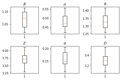
I risultati delle nostre inferenze. Noi tracciare i valori massima verosimiglianza per tutti i paramters globali per mostrare la loro variazione in tutte le nostre num_batches piste indipendenti di inferenza. Ciò corrisponde alla tabella S1 nei materiali supplementari.
fig, axs = plt.subplots(2, 3)
axs[0, 0].boxplot(best_parameters.documented_infectious_tx_rate,
                  whis=(2.5,97.5), sym='')
axs[0, 0].set_title(r'$\beta$')

axs[0, 1].boxplot(best_parameters.undocumented_infectious_tx_relative_rate,
                  whis=(2.5,97.5), sym='')
axs[0, 1].set_title(r'$\mu$')

axs[0, 2].boxplot(best_parameters.intercity_underreporting_factor,
                  whis=(2.5,97.5), sym='')
axs[0, 2].set_title(r'$\theta$')

axs[1, 0].boxplot(best_parameters.average_latency_period,
                  whis=(2.5,97.5), sym='')
axs[1, 0].set_title(r'$Z$')

axs[1, 1].boxplot(best_parameters.fraction_of_documented_infections,
                  whis=(2.5,97.5), sym='')
axs[1, 1].set_title(r'$\alpha$')

axs[1, 2].boxplot(best_parameters.average_infection_duration,
                  whis=(2.5,97.5), sym='')
axs[1, 2].set_title(r'$D$')
plt.tight_layout()