| | |  Kaynağı GitHub'da görüntüleyin Kaynağı GitHub'da görüntüleyin | |
Bu, Li ve diğerleri tarafından yazılan 16 Mart 2020 tarihli aynı isimli makalenin TensorFlow Olasılık bağlantı noktasıdır. Orijinal yazarların yöntemlerini ve sonuçlarını TensorFlow Probability platformunda aslına uygun olarak yeniden üreterek TFP'nin modern epidemiyoloji modellemesi ortamındaki bazı yeteneklerini sergiliyoruz. TensorFlow'a bağlantı bize orijinal Matlab koduna göre ~10x hızlanma sağlar ve TensorFlow Olasılığı vektörleştirilmiş toplu hesaplamayı yaygın olarak desteklediğinden, ayrıca yüzlerce bağımsız çoğaltmaya uygun şekilde ölçeklenir.
Orjinal kağıt
Ruiyun Li, Sen Pei, Bin Chen, Yimeng Song, Tao Zhang, Wan Yang ve Jeffrey Shaman. Önemli belgelenmemiş enfeksiyon, yeni koronavirüsün (SARS-CoV2) hızla yayılmasını kolaylaştırır. (2020 yılında), DOI: https://doi.org/10.1126/science.abb3221 .
Özet:. "Yaygınlık ve belgesiz roman coronavirüs (SARS-CoV2) enfeksiyonların bulaşıcılık tahmini genel yaygınlığını ve bu hastalığın salgın potansiyeli anlamak için kritik öneme sahiptir Burada hareketlilik verileri bir birlikte, Çin içinde raporlanan enfeksiyon gözlemlerini kullanmak Belgelenmemiş enfeksiyonların oranı ve bulaşıcılıkları dahil olmak üzere SARS-CoV2 ile ilişkili kritik epidemiyolojik özellikleri çıkarmak için ağ bağlantılı dinamik metapopülasyon modeli ve Bayes çıkarımı Tüm enfeksiyonların %86'sının belgesiz olduğunu tahmin ediyoruz (%95 GA: [%82-%90] ) 23 Ocak 2020 seyahat kısıtlamalarından önce Kişi başına, belgesiz enfeksiyonların bulaşma oranı belgelenmiş enfeksiyonların %55'iydi ([%46-%62]), ancak daha fazla sayıları nedeniyle, belgelenmemiş enfeksiyonlar 79 için enfeksiyon kaynağıydı Bu bulgular, SARS-CoV2'nin hızlı coğrafi yayılımını açıklıyor ve bu virüsün kontrol altına alınmasının özellikle zor olacağını gösteriyor."
Github bağlantı kodu ve verilere.
genel bakış
Model olduğu bölmeli hastalık modeli "duyarlı", "maruz" (enfekte ancak henüz bulaşıcı değil), "bulaşıcı belgelenmiş hiçbir zaman" ve "bulaşıcı sonunda belgelenmiş" için bölmeleri olan,. Dikkate değer iki özellik var: insanların bir şehirden diğerine nasıl seyahat ettiğine dair bir varsayımla 375 Çin şehrinin her biri için ayrı bölmeler; ve dönüşen bir vaka günde "bulaşıcı sonunda belgelenmiş" böylece enfeksiyon raporlama gecikmeler \(t\) bir stokastik sonra güne kadar gözlemlenen olgu sayılarında görünmüyor.
Model, hiçbir zaman belgelenmemiş vakaların daha hafif olmakla belgelenmediğini ve böylece diğerlerine daha düşük oranda bulaştığını varsayar. Orijinal makaledeki ana parametre, hem mevcut enfeksiyonun boyutunu hem de belgesiz bulaşmanın hastalığın yayılması üzerindeki etkisini tahmin etmek için belgesiz vakaların oranıdır.
Bu ortak çalışma, aşağıdan yukarıya stilde bir kod kılavuzu olarak yapılandırılmıştır. Sırayla, yapacağız
- Verileri alın ve kısaca inceleyin,
- Modelin durum uzayını ve dinamiklerini tanımlar,
- Li ve diğerlerini takip eden modelde çıkarım yapmak için bir dizi fonksiyon oluşturun ve
- Onları çağırın ve sonuçları inceleyin. Spoiler: Kağıtla aynı çıkıyorlar.
Kurulum ve Python İthalatları
pip3 install -q tf-nightly tfp-nightly
import collections
import io
import requests
import time
import zipfile

import matplotlib.pyplot as plt
import numpy as np
import pandas as pd

import tensorflow.compat.v2 as tf
import tensorflow_probability as tfp
from tensorflow_probability.python.internal import samplers

tfd = tfp.distributions
tfes = tfp.experimental.sequential
Veri İçe Aktarma
Verileri github'dan içe aktaralım ve bir kısmını inceleyelim.
r = requests.get('https://raw.githubusercontent.com/SenPei-CU/COVID-19/master/Data.zip')
z = zipfile.ZipFile(io.BytesIO(r.content))
z.extractall('/tmp/')
raw_incidence = pd.read_csv('/tmp/data/Incidence.csv')
raw_mobility = pd.read_csv('/tmp/data/Mobility.csv')
raw_population = pd.read_csv('/tmp/data/pop.csv')
Aşağıda günlük ham insidans sayısını görebiliriz. 23'ünde seyahat kısıtlamaları yürürlüğe girdiğinden, en çok ilk 14 gün (10 Ocak - 23 Ocak) ile ilgileniyoruz. Makale, 10-23 Ocak ve 23+ Ocak'ı farklı parametrelerle ayrı ayrı modelleyerek bu konuyu ele alıyor; ürememizi sadece önceki dönemle sınırlayacağız.
raw_incidence.drop('Date', axis=1)  # The 'Date' column is all 1/18/21
# Luckily the days are in order, starting on January 10th, 2020.
Wuhan insidansının sayılarını akıl sağlığıyla kontrol edelim.
plt.plot(raw_incidence.Wuhan, '.-')
plt.title('Wuhan incidence counts over 1/10/20 - 02/08/20')
plt.show()
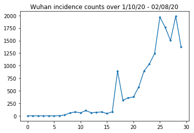
Çok uzak çok iyi. Şimdi ilk nüfus sayılır.
raw_population
Ayrıca hangi girişin Wuhan olduğunu kontrol edip kaydedelim.
raw_population['City'][169]
'Wuhan'
WUHAN_IDX = 169
Ve burada farklı şehirler arasındaki hareketlilik matrisini görüyoruz. Bu, ilk 14 gün içinde farklı şehirler arasında hareket eden insan sayısını temsil etmektedir. Tencent tarafından 2018 Ay Yeni Yılı sezonu için sağlanan GPS kayıtlarından derlenmiştir. Bazı bilinmeyen (çıkarsama tabi) sabit faktör olarak 2020 sezonunda Li vd modeli hareketlilik \(\theta\) zamanlarda bu.
raw_mobility
Son olarak, tüm bunları tüketebileceğimiz numpy dizilerine önişleyelim.
# The given populations are only "initial" because of intercity mobility during
# the holiday season.
initial_population = raw_population['Population'].to_numpy().astype(np.float32)
Hareketlilik verilerini [L, L, T] şeklinde bir Tensöre dönüştürün; burada L, konum sayısı ve T, zaman adımı sayısıdır.
daily_mobility_matrices = []
for i in range(1, 15):
  day_mobility = raw_mobility[raw_mobility['Day'] == i]

  # Make a matrix of daily mobilities.
  z = pd.crosstab(
      day_mobility.Origin,
      day_mobility.Destination,
      values=day_mobility['Mobility Index'], aggfunc='sum', dropna=False)

  # Include every city, even if there are no rows for some in the raw data on
  # some day.  This uses the sort order of `raw_population`.
  z = z.reindex(index=raw_population['City'], columns=raw_population['City'],
                fill_value=0)
  # Finally, fill any missing entries with 0. This means no mobility.
  z = z.fillna(0)
  daily_mobility_matrices.append(z.to_numpy())

mobility_matrix_over_time = np.stack(daily_mobility_matrices, axis=-1).astype(
    np.float32)
Son olarak gözlemlenen enfeksiyonları alın ve bir [L, T] tablosu yapın.
# Remove the date parameter and take the first 14 days.
observed_daily_infectious_count = raw_incidence.to_numpy()[:14, 1:]
observed_daily_infectious_count = np.transpose(
    observed_daily_infectious_count).astype(np.float32)
Ve şekilleri istediğimiz gibi elde ettiğimizi iki kez kontrol edin. Bir hatırlatma olarak, 375 şehir ve 14 gün ile çalışıyoruz.
print('Mobility Matrix over time should have shape (375, 375, 14): {}'.format(
    mobility_matrix_over_time.shape))
print('Observed Infectious should have shape (375, 14): {}'.format(
    observed_daily_infectious_count.shape))
print('Initial population should have shape (375): {}'.format(
    initial_population.shape))
Mobility Matrix over time should have shape (375, 375, 14): (375, 375, 14)
Observed Infectious should have shape (375, 14): (375, 14)
Initial population should have shape (375): (375,)
Durumu ve Parametreleri Tanımlama
Modelimizi tanımlamaya başlayalım. Biz ürer model bir çeşididir Seir modeli . Bu durumda, aşağıdaki zamanla değişen durumlara sahibiz:
- \(S\): Her şehirde hastalığa duyarlı insanların sayısı.
- \(E\): hastalığa maruz her bir şehirdeki insanların sayısı ancak bulaşıcı henüz değil. Biyolojik olarak bu, hastalığa yakalanmaya tekabül eder, çünkü maruz kalan tüm insanlar sonunda bulaşıcı hale gelir.
- \(I^u\): bulaşıcı ama belgesiz olan her bir şehirdeki insanların sayısı. Modelde bu aslında "asla belgelenmeyecek" anlamına gelir.
- \(I^r\): bulaşıcı ve bu şekilde belgelenen her biri şehirdeki insanların sayısı. Li ve arkadaşları modeli raporlama gecikmeleri, böylece \(I^r\) aslında "gelecekte bir noktada belgelendirilmesi ciddi yeterlidir durumda" gibi bir şey karşılık gelir.
Aşağıda göreceğimiz gibi, zaman içinde bir Topluluk ayarlı Kalman Filtresi (EAKF) çalıştırarak bu durumları çıkaracağız. EAKF'nin durum vektörü, bu miktarların her biri için bir şehir endeksli vektördür.
Model, aşağıdaki çıkarsanabilir global, zamanla değişmeyen parametrelere sahiptir:
- \(\beta\): nedeniyle belgelenen-enfeksiyöz bireylere iletim hızı.
- \(\mu\): nedeniyle belgesiz-enfeksiyöz bireylere göre iletim hızı. Bu ürün sayesinde hareket edecek \(\mu \beta\).
- \(\theta\): şehirlerarası hareketlilik faktörü. Bu, hareketlilik verilerinin eksik bildirilmesi (ve 2018'den 2020'ye kadar nüfus artışı için) için düzeltme yapan 1'den büyük bir faktördür.
- \(Z\): Ortalama kuluçka süresi (yani, "maruz kalır" halde süresi).
- \(\alpha\): Bu olacak kadar şiddetli enfeksiyonlar fraksiyonudur (sonunda) belgelenmiştir.
- \(D\): enfeksiyonların ortalama süresi (yani, her iki "bulaşıcı" halde süresi).
Durumlar için EAKF çevresinde bir Yinelemeli Filtreleme döngüsü ile bu parametreler için nokta tahminleri çıkaracağız.
Model ayrıca çıkarsanamayan sabitlere de bağlıdır:
- \(M\): şehirlerarası hareket matrisi. Bu zamana göre değişir ve verildiği varsayılır. O anlaşılmaktadır parametre tarafından ölçeklendirildiğini olduğunu hatırlayın \(\theta\) şehirler arasındaki gerçek nüfus hareketlerini vermek.
- \(N\): Her şehirdeki kişilerin toplam sayısı. Verilen ilk topluluklar alınır ve nüfusun zaman varyasyonu hareket numaraları hesaplanır \(\theta M\).
İlk olarak, durumlarımızı ve parametrelerimizi tutmak için kendimize bazı veri yapıları veriyoruz.
SEIRComponents = collections.namedtuple(
  typename='SEIRComponents',
  field_names=[
    'susceptible',              # S
    'exposed',                  # E
    'documented_infectious',    # I^r
    'undocumented_infectious',  # I^u
    # This is the count of new cases in the "documented infectious" compartment.
    # We need this because we will introduce a reporting delay, between a person
    # entering I^r and showing up in the observable case count data.
    # This can't be computed from the cumulative `documented_infectious` count,
    # because some portion of that population will move to the 'recovered'
    # state, which we aren't tracking explicitly.
    'daily_new_documented_infectious'])

ModelParams = collections.namedtuple(
    typename='ModelParams',
    field_names=[
      'documented_infectious_tx_rate',             # Beta
      'undocumented_infectious_tx_relative_rate',  # Mu
      'intercity_underreporting_factor',           # Theta
      'average_latency_period',                    # Z
      'fraction_of_documented_infections',         # Alpha
      'average_infection_duration'                 # D
    ]
)
Ayrıca parametre değerleri için Li ve arkadaşlarının sınırlarını da kodluyoruz.
PARAMETER_LOWER_BOUNDS = ModelParams(
    documented_infectious_tx_rate=0.8,
    undocumented_infectious_tx_relative_rate=0.2,
    intercity_underreporting_factor=1.,
    average_latency_period=2.,
    fraction_of_documented_infections=0.02,
    average_infection_duration=2.
)

PARAMETER_UPPER_BOUNDS = ModelParams(
    documented_infectious_tx_rate=1.5,
    undocumented_infectious_tx_relative_rate=1.,
    intercity_underreporting_factor=1.75,
    average_latency_period=5.,
    fraction_of_documented_infections=1.,
    average_infection_duration=5.
)
SEIR Dinamikleri
Burada parametreler ve durum arasındaki ilişkiyi tanımlarız.
Li ve diğerlerinin zaman dinamiği denklemleri (tamamlayıcı malzeme, denklem 1-5) aşağıdaki gibidir:
\(\frac{dS_i}{dt} = -\beta \frac{S_i I_i^r}{N_i} - \mu \beta \frac{S_i I_i^u}{N_i} + \theta \sum_k \frac{M_{ij} S_j}{N_j - I_j^r} - + \theta \sum_k \frac{M_{ji} S_j}{N_i - I_i^r}\)
\(\frac{dE_i}{dt} = \beta \frac{S_i I_i^r}{N_i} + \mu \beta \frac{S_i I_i^u}{N_i} -\frac{E_i}{Z} + \theta \sum_k \frac{M_{ij} E_j}{N_j - I_j^r} - + \theta \sum_k \frac{M_{ji} E_j}{N_i - I_i^r}\)
\(\frac{dI^r_i}{dt} = \alpha \frac{E_i}{Z} - \frac{I_i^r}{D}\)
\(\frac{dI^u_i}{dt} = (1 - \alpha) \frac{E_i}{Z} - \frac{I_i^u}{D} + \theta \sum_k \frac{M_{ij} I_j^u}{N_j - I_j^r} - + \theta \sum_k \frac{M_{ji} I^u_j}{N_i - I_i^r}\)
\(N_i = N_i + \theta \sum_j M_{ij} - \theta \sum_j M_{ji}\)
Hatırlatma açısından \(i\) ve \(j\) indisler endeksi şehirler. Bu denklemler, hastalığın zaman evrimini modellemektedir.
- Daha fazla enfeksiyona yol açan bulaşıcı bireylerle temas;
- "Maruz kalma" durumundan "bulaşıcı" durumlardan birine hastalık ilerlemesi;
- Modellenen popülasyondan çıkararak modellediğimiz "bulaşıcı" durumlardan iyileşmeye doğru hastalık ilerlemesi;
- Maruz kalan veya belgesiz bulaşıcı kişiler dahil olmak üzere şehirler arası hareketlilik; ve
- Şehirler arası hareketlilik yoluyla günlük şehir nüfuslarının zamana göre değişimi.
Li ve arkadaşlarının ardından, sonunda rapor edilecek kadar şiddetli vakaları olan kişilerin şehirler arasında seyahat etmediğini varsayıyoruz.
Ayrıca Li ve diğerlerini izleyerek, bu dinamikleri terim bazında Poisson gürültüsüne tabi olarak ele alıyoruz, yani her terim aslında bir Poisson oranıdır, bir örnek içinden gerçek değişimi verir. Poisson gürültüsü terime dayalıdır, çünkü Poisson örneklerinin çıkarılması (eklemek yerine) Poisson dağıtılmış bir sonuç vermez.
Klasik dördüncü dereceden Runge-Kutta entegratörü ile bu dinamikleri zaman içinde ileriye doğru geliştireceğiz, ancak önce onları hesaplayan işlevi tanımlayalım (Poisson gürültüsünü örnekleme dahil).
def sample_state_deltas(
    state, population, mobility_matrix, params, seed, is_deterministic=False):
  """Computes one-step change in state, including Poisson sampling.

  Note that this is coded to support vectorized evaluation on arbitrary-shape
  batches of states.  This is useful, for example, for running multiple
  independent replicas of this model to compute credible intervals for the
  parameters.  We refer to the arbitrary batch shape with the conventional
  `B` in the parameter documentation below.  This function also, of course,
  supports broadcasting over the batch shape.

  Args:
    state: A `SEIRComponents` tuple with fields Tensors of shape
      B + [num_locations] giving the current disease state.
    population: A Tensor of shape B + [num_locations] giving the current city
      populations.
    mobility_matrix: A Tensor of shape B + [num_locations, num_locations] giving
      the current baseline inter-city mobility.
    params: A `ModelParams` tuple with fields Tensors of shape B giving the
      global parameters for the current EAKF run.
    seed: Initial entropy for pseudo-random number generation.  The Poisson
      sampling is repeatable by supplying the same seed.
    is_deterministic: A `bool` flag to turn off Poisson sampling if desired.

  Returns:
    delta: A `SEIRComponents` tuple with fields Tensors of shape
      B + [num_locations] giving the one-day changes in the state, according
      to equations 1-4 above (including Poisson noise per Li et al).
  """
  undocumented_infectious_fraction = state.undocumented_infectious / population
  documented_infectious_fraction = state.documented_infectious / population

  # Anyone not documented as infectious is considered mobile
  mobile_population = (population - state.documented_infectious)
  def compute_outflow(compartment_population):
    raw_mobility = tf.linalg.matvec(
        mobility_matrix, compartment_population / mobile_population)
    return params.intercity_underreporting_factor * raw_mobility
  def compute_inflow(compartment_population):
    raw_mobility = tf.linalg.matmul(
        mobility_matrix,
        (compartment_population / mobile_population)[..., tf.newaxis],
        transpose_a=True)
    return params.intercity_underreporting_factor * tf.squeeze(
        raw_mobility, axis=-1)

  # Helper for sampling the Poisson-variate terms.
  seeds = samplers.split_seed(seed, n=11)
  if is_deterministic:
    def sample_poisson(rate):
      return rate
  else:
    def sample_poisson(rate):
      return tfd.Poisson(rate=rate).sample(seed=seeds.pop())

  # Below are the various terms called U1-U12 in the paper. We combined the
  # first two, which should be fine; both are poisson so their sum is too, and
  # there's no risk (as there could be in other terms) of going negative.
  susceptible_becoming_exposed = sample_poisson(
      state.susceptible *
      (params.documented_infectious_tx_rate *
       documented_infectious_fraction +
       (params.undocumented_infectious_tx_relative_rate *
        params.documented_infectious_tx_rate) *
       undocumented_infectious_fraction))  # U1 + U2

  susceptible_population_inflow = sample_poisson(
      compute_inflow(state.susceptible))  # U3
  susceptible_population_outflow = sample_poisson(
      compute_outflow(state.susceptible))  # U4

  exposed_becoming_documented_infectious = sample_poisson(
      params.fraction_of_documented_infections *
      state.exposed / params.average_latency_period)  # U5
  exposed_becoming_undocumented_infectious = sample_poisson(
      (1 - params.fraction_of_documented_infections) *
      state.exposed / params.average_latency_period)  # U6

  exposed_population_inflow = sample_poisson(
      compute_inflow(state.exposed))  # U7
  exposed_population_outflow = sample_poisson(
      compute_outflow(state.exposed))  # U8

  documented_infectious_becoming_recovered = sample_poisson(
      state.documented_infectious /
      params.average_infection_duration)  # U9
  undocumented_infectious_becoming_recovered = sample_poisson(
      state.undocumented_infectious /
      params.average_infection_duration)  # U10

  undocumented_infectious_population_inflow = sample_poisson(
      compute_inflow(state.undocumented_infectious))  # U11
  undocumented_infectious_population_outflow = sample_poisson(
      compute_outflow(state.undocumented_infectious))  # U12

  # The final state_deltas
  return SEIRComponents(
      # Equation [1]
      susceptible=(-susceptible_becoming_exposed +
                   susceptible_population_inflow +
                   -susceptible_population_outflow),
      # Equation [2]
      exposed=(susceptible_becoming_exposed +
               -exposed_becoming_documented_infectious +
               -exposed_becoming_undocumented_infectious +
               exposed_population_inflow +
               -exposed_population_outflow),
      # Equation [3]
      documented_infectious=(
          exposed_becoming_documented_infectious +
          -documented_infectious_becoming_recovered),
      # Equation [4]
      undocumented_infectious=(
          exposed_becoming_undocumented_infectious +
          -undocumented_infectious_becoming_recovered +
          undocumented_infectious_population_inflow +
          -undocumented_infectious_population_outflow),
      # New to-be-documented infectious cases, subject to the delayed
      # observation model.
      daily_new_documented_infectious=exposed_becoming_documented_infectious)
İşte entegratör. Bu kadar PRNG tohum geçen haricinde tamamen standart sample_state_deltas Runge Kutta yöntem çağrıları kısmi adımların her biri bağımsız Poisson gürültü elde etmek için işlev görmektedir.
@tf.function(autograph=False)
def rk4_one_step(state, population, mobility_matrix, params, seed):
  """Implement one step of RK4, wrapped around a call to sample_state_deltas."""
  # One seed for each RK sub-step
  seeds = samplers.split_seed(seed, n=4)

  deltas = tf.nest.map_structure(tf.zeros_like, state)
  combined_deltas = tf.nest.map_structure(tf.zeros_like, state)

  for a, b in zip([1., 2, 2, 1.], [6., 3., 3., 6.]):
    next_input = tf.nest.map_structure(
        lambda x, delta, a=a: x + delta / a, state, deltas)
    deltas = sample_state_deltas(
        next_input,
        population,
        mobility_matrix,
        params,
        seed=seeds.pop(), is_deterministic=False)
    combined_deltas = tf.nest.map_structure(
        lambda x, delta, b=b: x + delta / b, combined_deltas, deltas)

  return tf.nest.map_structure(
      lambda s, delta: s + tf.round(delta),
      state, combined_deltas)
başlatma
Burada kağıttan başlatma şemasını uyguluyoruz.
Li ve arkadaşlarının ardından, çıkarım şemamız, yinelenen bir filtreleme dış döngüsü (IF-EAKF) ile çevrili bir topluluk ayarı Kalman filtresi iç döngüsü olacaktır. Hesaplamalı olarak, bu, üç tür başlatmaya ihtiyacımız olduğu anlamına gelir:
- İç EAKF için başlangıç durumu
- İlk EAKF için de başlangıç parametreleri olan dış IF için başlangıç parametreleri
- İlki dışındaki her EAKF için başlangıç parametreleri olarak hizmet eden, bir IF yinelemesinden diğerine parametreleri güncelleme.
def initialize_state(num_particles, num_batches, seed):
  """Initialize the state for a batch of EAKF runs.

  Args:
    num_particles: `int` giving the number of particles for the EAKF.
    num_batches: `int` giving the number of independent EAKF runs to
      initialize in a vectorized batch.
    seed: PRNG entropy.

  Returns:
    state: A `SEIRComponents` tuple with Tensors of shape [num_particles,
      num_batches, num_cities] giving the initial conditions in each
      city, in each filter particle, in each batch member.
  """
  num_cities = mobility_matrix_over_time.shape[-2]
  state_shape = [num_particles, num_batches, num_cities]
  susceptible = initial_population * np.ones(state_shape, dtype=np.float32)
  documented_infectious = np.zeros(state_shape, dtype=np.float32)
  daily_new_documented_infectious = np.zeros(state_shape, dtype=np.float32)

  # Following Li et al, initialize Wuhan with up to 2000 people exposed
  # and another up to 2000 undocumented infectious.
  rng = np.random.RandomState(seed[0] % (2**31 - 1))
  wuhan_exposed = rng.randint(
      0, 2001, [num_particles, num_batches]).astype(np.float32)
  wuhan_undocumented_infectious = rng.randint(
      0, 2001, [num_particles, num_batches]).astype(np.float32)

  # Also following Li et al, initialize cities adjacent to Wuhan with three
  # days' worth of additional exposed and undocumented-infectious cases,
  # as they may have traveled there before the beginning of the modeling
  # period.
  exposed = 3 * mobility_matrix_over_time[
      WUHAN_IDX, :, 0] * wuhan_exposed[
          ..., np.newaxis] / initial_population[WUHAN_IDX]
  undocumented_infectious = 3 * mobility_matrix_over_time[
      WUHAN_IDX, :, 0] * wuhan_undocumented_infectious[
          ..., np.newaxis] / initial_population[WUHAN_IDX]

  exposed[..., WUHAN_IDX] = wuhan_exposed
  undocumented_infectious[..., WUHAN_IDX] = wuhan_undocumented_infectious

  # Following Li et al, we do not remove the inital exposed and infectious
  # persons from the susceptible population.
  return SEIRComponents(
      susceptible=tf.constant(susceptible),
      exposed=tf.constant(exposed),
      documented_infectious=tf.constant(documented_infectious),
      undocumented_infectious=tf.constant(undocumented_infectious),
      daily_new_documented_infectious=tf.constant(daily_new_documented_infectious))

def initialize_params(num_particles, num_batches, seed):
  """Initialize the global parameters for the entire inference run.

  Args:
    num_particles: `int` giving the number of particles for the EAKF.
    num_batches: `int` giving the number of independent EAKF runs to
      initialize in a vectorized batch.
    seed: PRNG entropy.

  Returns:
    params: A `ModelParams` tuple with fields Tensors of shape
      [num_particles, num_batches] giving the global parameters
      to use for the first batch of EAKF runs.
  """
  # We have 6 parameters. We'll initialize with a Sobol sequence,
  # covering the hyper-rectangle defined by our parameter limits.
  halton_sequence = tfp.mcmc.sample_halton_sequence(
      dim=6, num_results=num_particles * num_batches, seed=seed)
  halton_sequence = tf.reshape(
      halton_sequence, [num_particles, num_batches, 6])
  halton_sequences = tf.nest.pack_sequence_as(
      PARAMETER_LOWER_BOUNDS, tf.split(
          halton_sequence, num_or_size_splits=6, axis=-1))
  def interpolate(minval, maxval, h):
    return (maxval - minval) * h + minval
  return tf.nest.map_structure(
      interpolate,
      PARAMETER_LOWER_BOUNDS, PARAMETER_UPPER_BOUNDS, halton_sequences)

def update_params(num_particles, num_batches,
                  prev_params, parameter_variance, seed):
  """Update the global parameters between EAKF runs.

  Args:
    num_particles: `int` giving the number of particles for the EAKF.
    num_batches: `int` giving the number of independent EAKF runs to
      initialize in a vectorized batch.
    prev_params: A `ModelParams` tuple of the parameters used for the previous
      EAKF run.
    parameter_variance: A `ModelParams` tuple specifying how much to drift
      each parameter.
    seed: PRNG entropy.

  Returns:
    params: A `ModelParams` tuple with fields Tensors of shape
      [num_particles, num_batches] giving the global parameters
      to use for the next batch of EAKF runs.
  """
  # Initialize near the previous set of parameters. This is the first step
  # in Iterated Filtering.
  seeds = tf.nest.pack_sequence_as(
      prev_params, samplers.split_seed(seed, n=len(prev_params)))
  return tf.nest.map_structure(
      lambda x, v, seed: x + tf.math.sqrt(v) * tf.random.stateless_normal([
          num_particles, num_batches, 1], seed=seed),
      prev_params, parameter_variance, seeds)
gecikmeler
Bu modelin önemli özelliklerinden biri, enfeksiyonların başladıktan sonra rapor edildiğinin açık bir şekilde dikkate alınmasıdır. Yani, biz dan hareket eden bir kişi bekliyoruz olduğu \(E\) için bölmeye \(I^r\) gün bölmeye \(t\) daha sonraki güne kadar gözlemlenebilir raporlanan vaka sayılarında görünmeyebilir.
Gecikmenin gama-dağıtılmış olduğunu varsayıyoruz. Li ve diğerlerini takiben, şekil için 1,85 kullanıyoruz ve ortalama 9 günlük bir raporlama gecikmesi üretmek için oranı parametreleştiriyoruz.
def raw_reporting_delay_distribution(gamma_shape=1.85, reporting_delay=9.):
  return tfp.distributions.Gamma(
      concentration=gamma_shape, rate=gamma_shape / reporting_delay)
Gözlemlerimiz kesiklidir, bu nedenle ham (sürekli) gecikmeleri en yakın güne yuvarlayacağız. Ayrıca sınırlı bir veri ufkumuz var, bu nedenle tek bir kişi için gecikme dağılımı kalan günlere göre kategoriktir. Bu nedenle örnekleme daha verimli başına kent tahmin gözlemler hesaplayabilir \(O(I^r)\) yerine ön-hesaplanması multinomial gecikme olasılıkları tarafından, gamaları.
def reporting_delay_probs(num_timesteps, gamma_shape=1.85, reporting_delay=9.):
  gamma_dist = raw_reporting_delay_distribution(gamma_shape, reporting_delay)
  multinomial_probs = [gamma_dist.cdf(1.)]
  for k in range(2, num_timesteps + 1):
    multinomial_probs.append(gamma_dist.cdf(k) - gamma_dist.cdf(k - 1))
  # For samples that are larger than T.
  multinomial_probs.append(gamma_dist.survival_function(num_timesteps))
  multinomial_probs = tf.stack(multinomial_probs)
  return multinomial_probs
İşte bu gecikmeleri günlük olarak belgelenmiş yeni bulaşıcı sayımlara gerçekten uygulamak için kod:
def delay_reporting(
    daily_new_documented_infectious, num_timesteps, t, multinomial_probs, seed):
  # This is the distribution of observed infectious counts from the current
  # timestep.

  raw_delays = tfd.Multinomial(
      total_count=daily_new_documented_infectious,
      probs=multinomial_probs).sample(seed=seed)

  # The last bucket is used for samples that are out of range of T + 1. Thus
  # they are not going to be observable in this model.
  clipped_delays = raw_delays[..., :-1]

  # We can also remove counts that are such that t + i >= T.
  clipped_delays = clipped_delays[..., :num_timesteps - t]
  # We finally shift everything by t. That means prepending with zeros.
  return tf.concat([
      tf.zeros(
          tf.concat([
              tf.shape(clipped_delays)[:-1], [t]], axis=0),
          dtype=clipped_delays.dtype),
      clipped_delays], axis=-1)
çıkarım
İlk önce çıkarım için bazı veri yapılarını tanımlayacağız.
Özellikle, çıkarım yaparken durumu ve parametreleri birlikte paketleyen Yinelemeli Filtreleme yapmak isteyeceğiz. Bu yüzden bir tanımlayacağız ParameterStatePair nesnesi.
Ayrıca herhangi bir yan bilgiyi modele paketlemek istiyoruz.
ParameterStatePair = collections.namedtuple(
    'ParameterStatePair', ['state', 'params'])

# Info that is tracked and mutated but should not have inference performed over.
SideInfo = collections.namedtuple(
    'SideInfo', [
        # Observations at every time step.
        'observations_over_time',
        'initial_population',
        'mobility_matrix_over_time',
        'population',
        # Used for variance of measured observations.
        'actual_reported_cases',
        # Pre-computed buckets for the multinomial distribution.
        'multinomial_probs',
        'seed',
    ])

# Cities can not fall below this fraction of people
MINIMUM_CITY_FRACTION = 0.6

# How much to inflate the covariance by.
INFLATION_FACTOR = 1.1

INFLATE_FN = tfes.inflate_by_scaled_identity_fn(INFLATION_FACTOR)
İşte Ensemble Kalman Filtresi için paketlenmiş tam gözlem modeli.
İlginç olan özellik, raporlama gecikmeleridir (önceden hesaplandığı gibi). Memba modeli yayar daily_new_documented_infectious her adımda her şehir için.
# We observe the observed infections.
def observation_fn(t, state_params, extra):
  """Generate reported cases.

  Args:
    state_params: A `ParameterStatePair` giving the current parameters
      and state.
    t: Integer giving the current time.
    extra: A `SideInfo` carrying auxiliary information.

  Returns:
    observations: A Tensor of predicted observables, namely new cases
      per city at time `t`.
    extra: Update `SideInfo`.
  """
  # Undo padding introduced in `inference`.
  daily_new_documented_infectious = state_params.state.daily_new_documented_infectious[..., 0]
  # Number of people that we have already committed to become
  # observed infectious over time.
  # shape: batch + [num_particles, num_cities, time]
  observations_over_time = extra.observations_over_time
  num_timesteps = observations_over_time.shape[-1]

  seed, new_seed = samplers.split_seed(extra.seed, salt='reporting delay')

  daily_delayed_counts = delay_reporting(
      daily_new_documented_infectious, num_timesteps, t,
      extra.multinomial_probs, seed)
  observations_over_time = observations_over_time + daily_delayed_counts

  extra = extra._replace(
      observations_over_time=observations_over_time,
      seed=new_seed)

  # Actual predicted new cases, re-padded.
  adjusted_observations = observations_over_time[..., t][..., tf.newaxis]
  # Finally observations have variance that is a function of the true observations:
  return tfd.MultivariateNormalDiag(
      loc=adjusted_observations,
      scale_diag=tf.math.maximum(
          2., extra.actual_reported_cases[..., t][..., tf.newaxis] / 2.)), extra
Burada geçiş dinamiklerini tanımlıyoruz. Anlamsal çalışmayı zaten yaptık; burada sadece EAKF çerçevesi için paketliyoruz ve Li ve diğerlerini izleyerek şehir nüfuslarını çok küçülmelerini önlemek için kırpıyoruz.
def transition_fn(t, state_params, extra):
  """SEIR dynamics.

  Args:
    state_params: A `ParameterStatePair` giving the current parameters
      and state.
    t: Integer giving the current time.
    extra: A `SideInfo` carrying auxiliary information.

  Returns:
    state_params: A `ParameterStatePair` predicted for the next time step.
    extra: Updated `SideInfo`.
  """
  mobility_t = extra.mobility_matrix_over_time[..., t]
  new_seed, rk4_seed = samplers.split_seed(extra.seed, salt='Transition')
  new_state = rk4_one_step(
      state_params.state,
      extra.population,
      mobility_t,
      state_params.params,
      seed=rk4_seed)

  # Make sure population doesn't go below MINIMUM_CITY_FRACTION.
  new_population = (
      extra.population + state_params.params.intercity_underreporting_factor * (
          # Inflow
          tf.reduce_sum(mobility_t, axis=-2) -
          # Outflow
          tf.reduce_sum(mobility_t, axis=-1)))
  new_population = tf.where(
      new_population < MINIMUM_CITY_FRACTION * extra.initial_population,
      extra.initial_population * MINIMUM_CITY_FRACTION,
      new_population)

  extra = extra._replace(population=new_population, seed=new_seed)

  # The Ensemble Kalman Filter code expects the transition function to return a distribution.
  # As the dynamics and noise are encapsulated above, we construct a `JointDistribution` that when
  # sampled, returns the values above.

  new_state = tfd.JointDistributionNamed(
      model=tf.nest.map_structure(lambda x: tfd.VectorDeterministic(x), new_state))
  params = tfd.JointDistributionNamed(
      model=tf.nest.map_structure(lambda x: tfd.VectorDeterministic(x), state_params.params))

  state_params = tfd.JointDistributionNamed(
      model=ParameterStatePair(state=new_state, params=params))

  return state_params, extra
Son olarak çıkarım yöntemini tanımlıyoruz. Bu iki döngüdür, dış döngü Yinelenen Filtreleme, iç döngü ise Topluluk Ayarlama Kalman Filtrelemedir.
# Use tf.function to speed up EAKF prediction and updates.
ensemble_kalman_filter_predict = tf.function(
    tfes.ensemble_kalman_filter_predict, autograph=False)
ensemble_adjustment_kalman_filter_update = tf.function(
    tfes.ensemble_adjustment_kalman_filter_update, autograph=False)

def inference(
    num_ensembles,
    num_batches,
    num_iterations,
    actual_reported_cases,
    mobility_matrix_over_time,
    seed=None,
    # This is how much to reduce the variance by in every iterative
    # filtering step.
    variance_shrinkage_factor=0.9,
    # Days before infection is reported.
    reporting_delay=9.,
    # Shape parameter of Gamma distribution.
    gamma_shape_parameter=1.85):
  """Inference for the Shaman, et al. model.

  Args:
    num_ensembles: Number of particles to use for EAKF.
    num_batches: Number of batches of IF-EAKF to run.
    num_iterations: Number of iterations to run iterative filtering.
    actual_reported_cases: `Tensor` of shape `[L, T]` where `L` is the number
      of cities, and `T` is the timesteps.
    mobility_matrix_over_time: `Tensor` of shape `[L, L, T]` which specifies the
      mobility between locations over time.
    variance_shrinkage_factor: Python `float`. How much to reduce the
      variance each iteration of iterated filtering.
    reporting_delay: Python `float`. How many days before the infection
      is reported.
    gamma_shape_parameter: Python `float`. Shape parameter of Gamma distribution
      of reporting delays.

  Returns:
    result: A `ModelParams` with fields Tensors of shape [num_batches],
      containing the inferred parameters at the final iteration.
  """
  print('Starting inference.')
  num_timesteps = actual_reported_cases.shape[-1]
  params_per_iter = []

  multinomial_probs = reporting_delay_probs(
      num_timesteps, gamma_shape_parameter, reporting_delay)

  seed = samplers.sanitize_seed(seed, salt='Inference')

  for i in range(num_iterations):
    start_if_time = time.time()
    seeds = samplers.split_seed(seed, n=4, salt='Initialize')
    if params_per_iter:
      parameter_variance = tf.nest.map_structure(
          lambda minval, maxval: variance_shrinkage_factor ** (
              2 * i) * (maxval - minval) ** 2 / 4.,
          PARAMETER_LOWER_BOUNDS, PARAMETER_UPPER_BOUNDS)
      params_t = update_params(
          num_ensembles,
          num_batches,
          prev_params=params_per_iter[-1],
          parameter_variance=parameter_variance,
          seed=seeds.pop())
    else:
      params_t = initialize_params(num_ensembles, num_batches, seed=seeds.pop())

    state_t = initialize_state(num_ensembles, num_batches, seed=seeds.pop())
    population_t = sum(x for x in state_t)
    observations_over_time = tf.zeros(
        [num_ensembles,
         num_batches,
         actual_reported_cases.shape[0], num_timesteps])

    extra = SideInfo(
        observations_over_time=observations_over_time,
        initial_population=tf.identity(population_t),
        mobility_matrix_over_time=mobility_matrix_over_time,
        population=population_t,
        multinomial_probs=multinomial_probs,
        actual_reported_cases=actual_reported_cases,
        seed=seeds.pop())

    # Clip states
    state_t = clip_state(state_t, population_t)
    params_t = clip_params(params_t, seed=seeds.pop())

    # Accrue the parameter over time. We'll be averaging that
    # and using that as our MLE estimate.
    params_over_time = tf.nest.map_structure(
        lambda x: tf.identity(x), params_t)

    state_params = ParameterStatePair(state=state_t, params=params_t)

    eakf_state = tfes.EnsembleKalmanFilterState(
        step=tf.constant(0), particles=state_params, extra=extra)

    for j in range(num_timesteps):
      seeds = samplers.split_seed(eakf_state.extra.seed, n=3)

      extra = extra._replace(seed=seeds.pop())

      # Predict step.

      # Inflate and clip.
      new_particles = INFLATE_FN(eakf_state.particles)
      state_t = clip_state(new_particles.state, eakf_state.extra.population)
      params_t = clip_params(new_particles.params, seed=seeds.pop())
      eakf_state = eakf_state._replace(
          particles=ParameterStatePair(params=params_t, state=state_t))

      eakf_predict_state = ensemble_kalman_filter_predict(eakf_state, transition_fn)

      # Clip the state and particles.
      state_params = eakf_predict_state.particles
      state_t = clip_state(
          state_params.state, eakf_predict_state.extra.population)
      state_params = ParameterStatePair(state=state_t, params=state_params.params)

      # We preprocess the state and parameters by affixing a 1 dimension. This is because for
      # inference, we treat each city as independent. We could also introduce localization by
      # considering cities that are adjacent.
      state_params = tf.nest.map_structure(lambda x: x[..., tf.newaxis], state_params)
      eakf_predict_state = eakf_predict_state._replace(particles=state_params)

      # Update step.

      eakf_update_state = ensemble_adjustment_kalman_filter_update(
          eakf_predict_state,
          actual_reported_cases[..., j][..., tf.newaxis],
          observation_fn)

      state_params = tf.nest.map_structure(
          lambda x: x[..., 0], eakf_update_state.particles)

      # Clip to ensure parameters / state are well constrained.
      state_t = clip_state(
          state_params.state, eakf_update_state.extra.population)

      # Finally for the parameters, we should reduce over all updates. We get
      # an extra dimension back so let's do that.
      params_t = tf.nest.map_structure(
          lambda x, y: x + tf.reduce_sum(y[..., tf.newaxis] - x, axis=-2, keepdims=True),
          eakf_predict_state.particles.params, state_params.params)
      params_t = clip_params(params_t, seed=seeds.pop())
      params_t = tf.nest.map_structure(lambda x: x[..., 0], params_t)

      state_params = ParameterStatePair(state=state_t, params=params_t)
      eakf_state = eakf_update_state
      eakf_state = eakf_state._replace(particles=state_params)

      # Flatten and collect the inferred parameter at time step t.
      params_over_time = tf.nest.map_structure(
          lambda s, x: tf.concat([s, x], axis=-1), params_over_time, params_t)

    est_params = tf.nest.map_structure(
        # Take the average over the Ensemble and over time.
        lambda x: tf.math.reduce_mean(x, axis=[0, -1])[..., tf.newaxis],
        params_over_time)
    params_per_iter.append(est_params)
    print('Iterated Filtering {} / {} Ran in: {:.2f} seconds'.format(
        i, num_iterations, time.time() - start_if_time))

  return tf.nest.map_structure(
      lambda x: tf.squeeze(x, axis=-1), params_per_iter[-1])
Son ayrıntı: parametreleri ve durumu kırpmak, bunların aralık dahilinde olduğundan ve negatif olmadığından emin olmaktan ibarettir.
def clip_state(state, population):
  """Clip state to sensible values."""
  state = tf.nest.map_structure(
      lambda x: tf.where(x < 0, 0., x), state)

  # If S > population, then adjust as well.
  susceptible = tf.where(state.susceptible > population, population, state.susceptible)
  return SEIRComponents(
      susceptible=susceptible,
      exposed=state.exposed,
      documented_infectious=state.documented_infectious,
      undocumented_infectious=state.undocumented_infectious,
      daily_new_documented_infectious=state.daily_new_documented_infectious)

def clip_params(params, seed):
  """Clip parameters to bounds."""
  def _clip(p, minval, maxval):
    return tf.where(
        p < minval,
        minval * (1. + 0.1 * tf.random.stateless_uniform(p.shape, seed=seed)),
        tf.where(p > maxval,
                 maxval * (1. - 0.1 * tf.random.stateless_uniform(
                     p.shape, seed=seed)), p))
  params = tf.nest.map_structure(
      _clip, params, PARAMETER_LOWER_BOUNDS, PARAMETER_UPPER_BOUNDS)

  return params
Hepsini bir arada yürütmek
# Let's sample the parameters.
#
# NOTE: Li et al. run inference 1000 times, which would take a few hours.
# Here we run inference 30 times (in a single, vectorized batch).
best_parameters = inference(
    num_ensembles=300,
    num_batches=30,
    num_iterations=10,
    actual_reported_cases=observed_daily_infectious_count,
    mobility_matrix_over_time=mobility_matrix_over_time)
Starting inference.
Iterated Filtering 0 / 10 Ran in: 26.65 seconds
Iterated Filtering 1 / 10 Ran in: 28.69 seconds
Iterated Filtering 2 / 10 Ran in: 28.06 seconds
Iterated Filtering 3 / 10 Ran in: 28.48 seconds
Iterated Filtering 4 / 10 Ran in: 28.57 seconds
Iterated Filtering 5 / 10 Ran in: 28.35 seconds
Iterated Filtering 6 / 10 Ran in: 28.35 seconds
Iterated Filtering 7 / 10 Ran in: 28.19 seconds
Iterated Filtering 8 / 10 Ran in: 28.58 seconds
Iterated Filtering 9 / 10 Ran in: 28.23 seconds
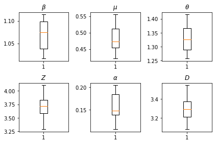
Çıkarımlarımızın sonuçları. Tüm global parametresinin tanımlanması bizim genelinde değişimi göstermek için biz maksimum olabilirlik değerlerini çizmek num_batches çıkarım bağımsız çalışır. Bu, ek materyallerdeki Tablo S1'e karşılık gelir.
fig, axs = plt.subplots(2, 3)
axs[0, 0].boxplot(best_parameters.documented_infectious_tx_rate,
                  whis=(2.5,97.5), sym='')
axs[0, 0].set_title(r'$\beta$')

axs[0, 1].boxplot(best_parameters.undocumented_infectious_tx_relative_rate,
                  whis=(2.5,97.5), sym='')
axs[0, 1].set_title(r'$\mu$')

axs[0, 2].boxplot(best_parameters.intercity_underreporting_factor,
                  whis=(2.5,97.5), sym='')
axs[0, 2].set_title(r'$\theta$')

axs[1, 0].boxplot(best_parameters.average_latency_period,
                  whis=(2.5,97.5), sym='')
axs[1, 0].set_title(r'$Z$')

axs[1, 1].boxplot(best_parameters.fraction_of_documented_infections,
                  whis=(2.5,97.5), sym='')
axs[1, 1].set_title(r'$\alpha$')

axs[1, 2].boxplot(best_parameters.average_infection_duration,
                  whis=(2.5,97.5), sym='')
axs[1, 2].set_title(r'$D$')
plt.tight_layout()