যৌথ বিতরণ সহ সম্ভাব্য গ্রাফিক্যাল মডেলগুলির উপর বৈচিত্র্যপূর্ণ অনুমান

TensorFlow.org এ দেখুন

Google Colab-এ চালান

GitHub-এ উৎস দেখুন

নোটবুক ডাউনলোড করুন

ভেরিয়েশনাল ইনফারেন্স (VI) একটি অপ্টিমাইজেশান সমস্যা হিসাবে আনুমানিক বায়েসিয়ান ইনফরেন্সকে কাস্ট করে এবং একটি 'সারোগেট' পোস্টেরিয়র ডিস্ট্রিবিউশন খোঁজে যা সত্যিকারের পোস্টেরিয়রের সাথে KL ডিভার্জেন্সকে কমিয়ে দেয়। গ্রেডিয়েন্ট-ভিত্তিক VI প্রায়শই MCMC পদ্ধতির চেয়ে দ্রুত, মডেলের পরামিতিগুলির অপ্টিমাইজেশনের সাথে স্বাভাবিকভাবেই রচনা করে এবং মডেলের প্রমাণের উপর একটি নিম্ন সীমা প্রদান করে যা মডেল তুলনা, অভিসার নির্ণয় এবং সংমিশ্রণযোগ্য অনুমানের জন্য সরাসরি ব্যবহার করা যেতে পারে।

TensorFlow সম্ভাব্যতা দ্রুত, নমনীয়, এবং স্কেলযোগ্য VI এর জন্য টুল অফার করে যা স্বাভাবিকভাবে TFP স্ট্যাকের সাথে ফিট করে। এই সরঞ্জামগুলি রৈখিক রূপান্তর বা প্রবাহকে স্বাভাবিক করার দ্বারা প্ররোচিত সহ-ভারসাম্য কাঠামোর সাথে সারোগেট পোস্টেরিয়র তৈরি করতে সক্ষম করে।

ষষ্ঠ Bayesian অনুমান করার জন্য ব্যবহার করা যেতে পারে বিশ্বাসযোগ্য অন্তর একটি রিগ্রেশন মডেল পরামিতি সুদের একটি ফলাফল বিভিন্ন চিকিত্সা বা পর্যবেক্ষিত বৈশিষ্ট্য প্রভাব অনুমান করার জন্য। পর্যবেক্ষিত ডেটার উপর শর্তযুক্ত পরামিতিটির পোস্টেরিয়র ডিস্ট্রিবিউশন অনুসারে এবং প্যারামিটারের পূর্বের বন্টনের উপর একটি অনুমান প্রদত্ত বিশ্বাসযোগ্য ব্যবধানগুলি একটি নির্দিষ্ট সম্ভাব্যতার সাথে একটি অপ্রদর্শিত প্যারামিটারের মানকে আবদ্ধ করে।

এই Colab, আমরা ষষ্ঠ কীভাবে ব্যবহার করবেন তা একটি Bayesian বাড়িতে মাপা রাডন স্তরের জন্য রিগ্রেশন মডেল রৈখিক পরামিতি জন্য বিশ্বাসযোগ্য অন্তর প্রাপ্ত প্রদর্শন (ব্যবহার Gelman এট এর (2007) রাডন ডেটা সেটটি। কিন্তু দেখ অনুরূপ উদাহরণ স্ট্যান মধ্যে)। আমরা প্রদর্শন কিভাবে TFP JointDistribution s এর সাথে মেশা bijectors বিল্ড প্রয়োজন এবং ভাবপূর্ণ ভাড়াটে অধোদেশ দুই ধরনের মাপসই:

• একটি ব্লক ম্যাট্রিক্স দ্বারা রূপান্তরিত একটি আদর্শ সাধারণ বিতরণ। ম্যাট্রিক্স পশ্চাদ্দেশের কিছু উপাদানের মধ্যে স্বাধীনতা এবং অন্যদের মধ্যে নির্ভরতা প্রতিফলিত করতে পারে, একটি গড়-ক্ষেত্র বা সম্পূর্ণ-কোভারিয়েন্স পোস্টেরিয়র অনুমানকে শিথিল করে।
• একটি আরো জটিল, উচ্চ-ক্ষমতা সম্পন্ন autoregressive প্রবাহ বিপরীত ।

সারোগেট পোস্টেরিয়রদের প্রশিক্ষণ দেওয়া হয় এবং একটি গড়-ক্ষেত্রের সারোগেট পোস্টেরিয়র বেসলাইনের ফলাফলের সাথে তুলনা করা হয়, সেইসাথে হ্যামিলটোনিয়ান মন্টে কার্লোর গ্রাউন্ড-ট্রুথ নমুনা।

বায়েসিয়ান ভেরিয়েশনাল ইনফারেন্সের ওভারভিউ

ধরুন আমরা নিম্নলিখিত সৃজক প্রক্রিয়া, যেখানে আছে \(\theta\) র্যান্ডম পরামিতি প্রতিনিধিত্ব করে, \(\omega\) নির্ণায়ক পরামিতি প্রতিনিধিত্ব করে আর \(x_i\) বৈশিষ্ট্য এবং \(y_i\) লক্ষ্য মানের জন্য হয় \(i=1,\ldots,n\) ডাটা পয়েন্টের পরিলক্ষিত: \ সারিবদ্ধ শুরু { } &\theta \sim r(\Theta) && \text{(Prior)}\ &\text{for } i = 1 \ldots n: \nonumber \ &\quad y_i \sim p(Y_i|x_i, \theta , \ ওমেগা) && \ টেক্সট {(সম্ভাবনা)} \ শেষ {সারিবদ্ধ}

VI এর দ্বারা চিহ্নিত করা হয়: $\newcommand{\E}{\operatorname{\mathbb{E} } } \newcommand{\K}{\operatorname{\mathbb{K} } } \newcommand{\defeq}{\overset {\tiny\text{def} }{=} } \DeclareMathOperator*{\argmin}{arg\,min}$

\ লগ পি ({y_i} _i ^ এন | {x_i} _i ^ এন, \ ওমেগা) - \ {সারিবদ্ধ} শুরু & \ defeq - \ লগ ইন করুন \ int- এ \ textrm {ঘ} \ থেটা \, দ (\ থেটা) \ prod_i^np(y_i|x_i,\theta, \omega) && \text{(সত্যিই কঠিন অবিচ্ছেদ্য)} \ &= -\log \int \textrm{d}\theta\, q(\theta) \frac{1 }{q(\theta)} r(\theta) \prod_i^np(y_i|x_i,\theta, \omega) && \text{(1 দ্বারা গুণ করুন)}\ &\le - \int \textrm{d} \ থেটা \, কুই (\ থেটা) \ লগ অর্থাত \ frac {R (\ থেটা) \ prod_i ^ NP (y_i | এক্স আমি, \ থেটা, \ ওমেগা)} {কুই (\ থেটা)} && \ টেক্সট {(জেনসেন এর বৈষম্য )} \ & \ defeq \ ই {কুই (\ theta)} [- \ লগ P (y_i | x_i, \ theta, \ ওমেগা)] \ k [কুই (\ theta), আর (\ theta)] \ & \ defeq \text{expected negative log likelihood"} + \ টেক্সট {কেএল regularizer"} \ শেষ {সারিবদ্ধ}

(টেকনিক্যালি আমরা অভিমানী করছি \(q\) হয় একেবারে একটানা থেকে সম্মান সঙ্গে \(r\)। আরও দেখুন, জেনসেন এর বৈষম্য ।)

যেহেতু সমস্ত q এর জন্য সীমাবদ্ধ, এটি স্পষ্টতই এর জন্য সবচেয়ে টাইট:

\[q^*,w^* = \argmin_{q \in \mathcal{Q},\omega\in\mathbb{R}^d} \left\{ \sum_i^n\E_{q(\Theta)}\left[ -\log p(y_i|x_i,\Theta, \omega) \right] + \K[q(\Theta), r(\Theta)] \right\}\]

পরিভাষা সংক্রান্ত, আমরা কল

• \(q^*\) "ভাড়াটে অবর" এবং,
• \(\mathcal{Q}\) "ভাড়াটে পরিবার।"

\(\omega^*\) ষষ্ঠ ক্ষতির নির্ণায়ক প্যারামিটার সর্বোচ্চ-সম্ভাবনা মান প্রতিনিধিত্ব করে। দেখুন এই জরিপ ভেরিয়েশনাল অনুমান সম্পর্কে আরও তথ্যের জন্য।

উদাহরণ: Radon পরিমাপের উপর Bayesian শ্রেণীবিন্যাস লিনিয়ার রিগ্রেশন

রেডন একটি তেজস্ক্রিয় গ্যাস যা মাটির সাথে যোগাযোগ বিন্দুর মাধ্যমে ঘরে প্রবেশ করে। এটি একটি কার্সিনোজেন যা অধূমপায়ীদের ফুসফুসের ক্যান্সারের প্রাথমিক কারণ। র‌্যাডনের মাত্রা পরিবার থেকে পরিবারে ব্যাপকভাবে পরিবর্তিত হয়।

EPA 80,000 বাড়িতে রেডন স্তরের একটি গবেষণা করেছে। দুটি গুরুত্বপূর্ণ ভবিষ্যদ্বাণী হল:

• যে মেঝেতে পরিমাপ করা হয়েছিল (বেসমেন্টে রেডন উচ্চতর)
• কাউন্টি ইউরেনিয়াম স্তর (রেডন স্তরের সাথে ইতিবাচক সম্পর্ক)

কাউন্টি দ্বারা দলবদ্ধ ঘরের মধ্যে রাডন মাত্রা প্রেডিক্টিং Bayesian হায়ারারকিকাল মডেলিং একটি ক্লাসিক সমস্যা, চালু হয় Gelman এবং হিল (2006) । আমরা ঘরগুলিতে রেডন পরিমাপের পূর্বাভাস দেওয়ার জন্য একটি শ্রেণিবদ্ধ রৈখিক মডেল তৈরি করব, যেখানে শ্রেণিবিন্যাস হল কাউন্টি অনুসারে ঘরগুলির গ্রুপিং। আমরা মিনেসোটাতে বাড়ির রেডন স্তরে অবস্থানের (কাউন্টি) প্রভাবের জন্য বিশ্বাসযোগ্য বিরতিতে আগ্রহী। এই প্রভাবকে বিচ্ছিন্ন করার জন্য, মেঝে এবং ইউরেনিয়াম স্তরের প্রভাবগুলিও মডেলটিতে অন্তর্ভুক্ত করা হয়েছে। অতিরিক্তভাবে, আমরা কাউন্টি অনুসারে যে গড় মেঝেতে পরিমাপ করা হয়েছিল তার সাথে সম্পর্কিত একটি প্রাসঙ্গিক প্রভাব অন্তর্ভুক্ত করব, যাতে যে মেঝেতে পরিমাপ নেওয়া হয়েছিল তার কাউন্টির মধ্যে যদি তারতম্য থাকে তবে এটি কাউন্টি প্রভাবের জন্য দায়ী করা হবে না।

pip3 install -q tf-nightly tfp-nightly

import matplotlib.pyplot as plt
import numpy as np
import seaborn as sns
import tensorflow as tf
import tensorflow_datasets as tfds
import tensorflow_probability as tfp
import warnings

tfd = tfp.distributions
tfb = tfp.bijectors

plt.rcParams['figure.facecolor'] = '1.'

# Load the Radon dataset from `tensorflow_datasets` and filter to data from
# Minnesota.
dataset = tfds.as_numpy(
    tfds.load('radon', split='train').filter(
        lambda x: x['features']['state'] == 'MN').batch(10**9))

# Dependent variable: Radon measurements by house.
dataset = next(iter(dataset))
radon_measurement = dataset['activity'].astype(np.float32)
radon_measurement[radon_measurement <= 0.] = 0.1
log_radon = np.log(radon_measurement)

# Measured uranium concentrations in surrounding soil.
uranium_measurement = dataset['features']['Uppm'].astype(np.float32)
log_uranium = np.log(uranium_measurement)

# County indicator.
county_strings = dataset['features']['county'].astype('U13')
unique_counties, county = np.unique(county_strings, return_inverse=True)
county = county.astype(np.int32)
num_counties = unique_counties.size

# Floor on which the measurement was taken.
floor_of_house = dataset['features']['floor'].astype(np.int32)

# Average floor by county (contextual effect).
county_mean_floor = []
for i in range(num_counties):
  county_mean_floor.append(floor_of_house[county == i].mean())
county_mean_floor = np.array(county_mean_floor, dtype=log_radon.dtype)
floor_by_county = county_mean_floor[county]

রিগ্রেশন মডেলটি নিম্নরূপ উল্লেখ করা হয়েছে:

\(\newcommand{\Normal}{\operatorname{\sf Normal} }\)শুরু \ {সারিবদ্ধ} এবং \ টেক্সট {uranium_weight} \ সিম \ স্বাভাবিক (0, 1) \ & \ টেক্সট {county_floor_weight} \ সিম \ স্বাভাবিক (0, 1) \ & \ টেক্সট {জন্য} ঞ = 1 \ ldots \text{num_counties}:\ &\quad \text{county_effect}_j \sim \Normal (0, \sigma_c)\ &\text{for } i = 1\ldots n:\ &\quad \mu_i = ( \ & \ চতুর্ভুজ \ চতুর্ভুজ \ টেক্সট {পক্ষপাত} \ & \ চতুর্ভুজ \ চতুর্ভুজ + + \ টেক্সট {কাউন্টি প্রভাব} {\ টেক্সট {কাউন্টি} _i} \ & \ চতুর্ভুজ \ চতুর্ভুজ + + \ টেক্সট {log_uranium} _i \ বার \ টেক্সট {uranium_weight } \ & \ চতুর্ভুজ \ চতুর্ভুজ + + \ টেক্সট {floor_of_house} _i \ বার \ টেক্সট {floor_weight} \ & \ চতুর্ভুজ \ চতুর্ভুজ + + \ টেক্সট {floor_by কাউন্টি} {\ টেক্সট {কাউন্টি} _i} \ বার \ টেক্সট {county_floor_weight}) \ & \ চতুর্ভুজ \ টেক্সট {log_radon} _i \ সিম \ সাধারন (\ mu_i, \ sigma_y) \ শেষ {সারিবদ্ধ} যা \(i\) ইনডেক্স পর্যবেক্ষণ এবং \(\text{county}_i\) হয় কাউন্টি যা \(i\)তম পর্যবেক্ষণ ছিল নেওয়া

আমরা ভৌগলিক বৈচিত্র ক্যাপচার করতে একটি কাউন্টি-স্তরের র্যান্ডম প্রভাব ব্যবহার করি। পরামিতি uranium_weight এবং county_floor_weight সম্ভাব্য অনুকরণে করা হয়, এবং floor_weight এবং ধ্রুব bias নির্ণায়ক হয়। এই মডেলিং পছন্দগুলি মূলত নির্বিচারে, এবং যুক্তিসঙ্গত জটিলতার একটি সম্ভাব্য মডেলের উপর VI প্রদর্শনের উদ্দেশ্যে তৈরি করা হয়। TFP সংশোধন এবং র্যান্ডম প্রভাব, রাডন ডেটা সেটটি ব্যবহার করে বহুস্তরীয় মডেলিং একটি পুঙ্খানুপুঙ্খ আলোচনার জন্য দেখুন বহুস্তরীয় মডেলিং প্রাইমার এবং ভেরিয়েশনাল ইনফিরেনস ব্যবহার জুতসই জেনারেলাইজড লিনিয়ার মিশ্র-প্রতিক্রিয়া মডেল ।

# Create variables for fixed effects.
floor_weight = tf.Variable(0.)
bias = tf.Variable(0.)

# Variables for scale parameters.
log_radon_scale = tfp.util.TransformedVariable(1., tfb.Exp())
county_effect_scale = tfp.util.TransformedVariable(1., tfb.Exp())

# Define the probabilistic graphical model as a JointDistribution.
@tfd.JointDistributionCoroutineAutoBatched
def model():
  uranium_weight = yield tfd.Normal(0., scale=1., name='uranium_weight')
  county_floor_weight = yield tfd.Normal(
      0., scale=1., name='county_floor_weight')
  county_effect = yield tfd.Sample(
      tfd.Normal(0., scale=county_effect_scale),
      sample_shape=[num_counties], name='county_effect')
  yield tfd.Normal(
      loc=(log_uranium * uranium_weight + floor_of_house* floor_weight
           + floor_by_county * county_floor_weight
           + tf.gather(county_effect, county, axis=-1)
           + bias),
      scale=log_radon_scale[..., tf.newaxis],
      name='log_radon') 

# Pin the observed `log_radon` values to model the un-normalized posterior.
target_model = model.experimental_pin(log_radon=log_radon)

অভিব্যক্তিমূলক সারোগেট পোস্টেরিয়র

এরপরে আমরা দুটি ভিন্ন ধরণের সারোগেট পোস্টেরিয়র সহ VI ব্যবহার করে এলোমেলো প্রভাবগুলির উত্তরীয় বিতরণ অনুমান করি:

• ব্লকওয়াইজ ম্যাট্রিক্স ট্রান্সফর্মেশন দ্বারা প্রবর্তিত কোভেরিয়েন্স স্ট্রাকচার সহ একটি সীমাবদ্ধ মাল্টিভেরিয়েট সাধারণ বন্টন।
• একজন বহুচলকীয় আদর্শ সাধারন বন্টনের একটি দ্বারা রুপান্তরিত ইনভার্স Autoregressive ফ্লো , যা বিভক্ত এবং অবর সমর্থনে মেলে পুনর্গঠন করা হয়।

মাল্টিভেরিয়েট নরমাল সারোগেট পোস্টেরিয়র

এই সারোগেট পোস্টেরিয়র তৈরি করতে, একটি প্রশিক্ষিত রৈখিক অপারেটর পোস্টেরিয়রের উপাদানগুলির মধ্যে পারস্পরিক সম্পর্ককে প্ররোচিত করতে ব্যবহৃত হয়।

# Determine the `event_shape` of the posterior, and calculate the size of each
# `event_shape` component. These determine the sizes of the components of the
# underlying standard Normal distribution, and the dimensions of the blocks in
# the blockwise matrix transformation.
event_shape = target_model.event_shape_tensor()
flat_event_shape = tf.nest.flatten(event_shape)
flat_event_size = tf.nest.map_structure(tf.reduce_prod, flat_event_shape)

# The `event_space_bijector` maps unconstrained values (in R^n) to the support
# of the prior -- we'll need this at the end to constrain Multivariate Normal
# samples to the prior's support.
event_space_bijector = target_model.experimental_default_event_space_bijector()

একটি নির্মানের JointDistribution ভেক্টর-মূল্যবান আদর্শ স্বাভাবিক উপাদান সঙ্গে সংশ্লিষ্ট পূর্বে উপাদান দ্বারা নির্ধারিত আকারের সঙ্গে। উপাদানগুলি ভেক্টর-মূল্যবান হওয়া উচিত যাতে তারা রৈখিক অপারেটর দ্বারা রূপান্তরিত হতে পারে।

base_standard_dist = tfd.JointDistributionSequential(
      [tfd.Sample(tfd.Normal(0., 1.), s) for s in flat_event_size])

একটি প্রশিক্ষিত ব্লকওয়াইজ নিম্ন-ত্রিভুজাকার রৈখিক অপারেটর তৈরি করুন। একটি (প্রশিক্ষণযোগ্য) ব্লকওয়াইজ ম্যাট্রিক্স ট্রান্সফরমেশন বাস্তবায়ন করতে এবং পোস্টেরিয়রের পারস্পরিক সম্পর্ক গঠনকে প্ররোচিত করতে আমরা এটিকে স্ট্যান্ডার্ড নরমাল ডিস্ট্রিবিউশনে প্রয়োগ করব।

Blockwise রৈখিক অপারেটর মধ্যেই একটি trainable পুরো ম্যাট্রিক্স ব্লক, অবর দুই উপাদান মধ্যে পূর্ণ সহভেদাংক প্রতিনিধিত্ব করে যখন শূন্য (অথবা একটি ব্লক None ) স্বাধীনতা প্রকাশ করেছে। তির্যকের ব্লকগুলি হয় নিম্ন-ত্রিভুজাকার বা তির্যক ম্যাট্রিক্স, যাতে পুরো ব্লক কাঠামোটি একটি নিম্ন-ত্রিভুজাকার ম্যাট্রিক্সের প্রতিনিধিত্ব করে।

বেস ডিস্ট্রিবিউশনে এই বাইজেক্টর প্রয়োগ করার ফলে নিম্ন-ত্রিভুজাকার ব্লক ম্যাট্রিক্সের সমান 0 এবং (চোলেস্কি-ফ্যাক্টরড) কোভেরিয়েন্স সহ একটি মাল্টিভেরিয়েট সাধারণ বন্টন হয়।

operators = (
    (tf.linalg.LinearOperatorDiag,),  # Variance of uranium weight (scalar).
    (tf.linalg.LinearOperatorFullMatrix,  # Covariance between uranium and floor-by-county weights.
     tf.linalg.LinearOperatorDiag),  # Variance of floor-by-county weight (scalar).
    (None,  # Independence between uranium weight and county effects.
     None,  #  Independence between floor-by-county and county effects.
     tf.linalg.LinearOperatorDiag)  # Independence among the 85 county effects.
    )

block_tril_linop = (
    tfp.experimental.vi.util.build_trainable_linear_operator_block(
        operators, flat_event_size))
scale_bijector = tfb.ScaleMatvecLinearOperatorBlock(block_tril_linop)

আদর্শ সাধারন বন্টনের জন্য রৈখিক অপারেটর প্রযুক্ত হবার পর, একটি বহু-অংশযুক্ত আবেদন Shift গড় অশূন্য মান নিতে অনুমতি bijector।

loc_bijector = tfb.JointMap(
    tf.nest.map_structure(
        lambda s: tfb.Shift(
            tf.Variable(tf.random.uniform(
                (s,), minval=-2., maxval=2., dtype=tf.float32))),
        flat_event_size))

স্কেল এবং অবস্থান বিজেক্টর সহ স্ট্যান্ডার্ড সাধারণ বন্টনকে রূপান্তর করে প্রাপ্ত মাল্টিভেরিয়েট সাধারণ বন্টন, পূর্বের সাথে মেলে এবং শেষ পর্যন্ত পূর্বের সমর্থনে সীমাবদ্ধ করা আবশ্যক।

# Reshape each component to match the prior, using a nested structure of
# `Reshape` bijectors wrapped in `JointMap` to form a multipart bijector.
reshape_bijector = tfb.JointMap(
    tf.nest.map_structure(tfb.Reshape, flat_event_shape))

# Restructure the flat list of components to match the prior's structure
unflatten_bijector = tfb.Restructure(
        tf.nest.pack_sequence_as(
            event_shape, range(len(flat_event_shape))))

এখন, এটি সব একসাথে রাখুন -- প্রশিক্ষনযোগ্য বাইজেক্টরকে একসাথে চেইন করুন এবং সারোগেট পোস্টেরিয়র তৈরি করতে বেস স্ট্যান্ডার্ড নরমাল ডিস্ট্রিবিউশনে প্রয়োগ করুন।

surrogate_posterior = tfd.TransformedDistribution(
    base_standard_dist,
    bijector = tfb.Chain(  # Note that the chained bijectors are applied in reverse order
        [
         event_space_bijector,  # constrain the surrogate to the support of the prior
         unflatten_bijector,  # pack the reshaped components into the `event_shape` structure of the posterior
         reshape_bijector,  # reshape the vector-valued components to match the shapes of the posterior components
         loc_bijector,  # allow for nonzero mean
         scale_bijector  # apply the block matrix transformation to the standard Normal distribution
         ]))

মাল্টিভেরিয়েট সাধারণ সারোগেট পোস্টেরিয়রকে প্রশিক্ষণ দিন।

optimizer = tf.optimizers.Adam(learning_rate=1e-2)
mvn_loss = tfp.vi.fit_surrogate_posterior(
    target_model.unnormalized_log_prob,
    surrogate_posterior,
    optimizer=optimizer,
    num_steps=10**4,
    sample_size=16,
    jit_compile=True)

mvn_samples = surrogate_posterior.sample(1000)
mvn_final_elbo = tf.reduce_mean(
    target_model.unnormalized_log_prob(*mvn_samples)
    - surrogate_posterior.log_prob(mvn_samples))

print('Multivariate Normal surrogate posterior ELBO: {}'.format(mvn_final_elbo))

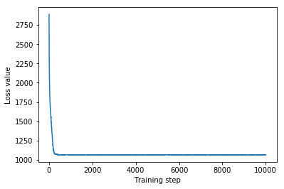
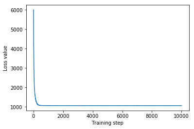
plt.plot(mvn_loss)
plt.xlabel('Training step')
_ = plt.ylabel('Loss value')

Multivariate Normal surrogate posterior ELBO: -1065.705322265625

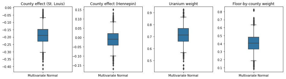
যেহেতু প্রশিক্ষিত সারোগেট পোস্টেরিয়র একটি TFP বিতরণ, আমরা এটি থেকে নমুনা নিতে পারি এবং পরামিতিগুলির জন্য পোস্টেরিয়র বিশ্বাসযোগ্য বিরতি তৈরি করতে সেগুলি প্রক্রিয়া করতে পারি।

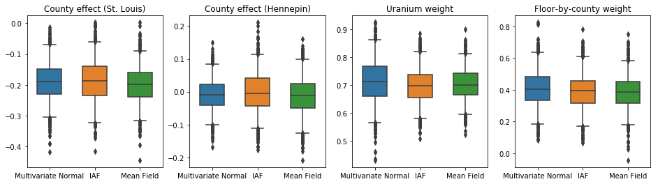
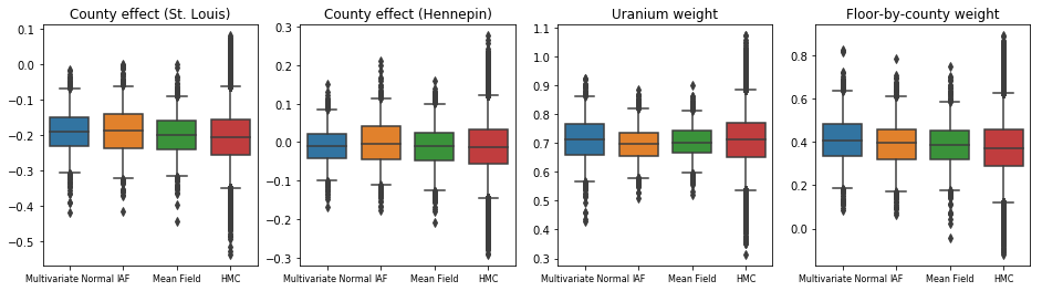
বক্স-এবং-গোঁফ প্লট নিচে 50% এবং 95% দেন বিশ্বাসযোগ্য অন্তর কাউন্টি কাউন্টি দ্বারা মাটি ইউরেনিয়াম পরিমাপের উপর দুই বৃহত্তম কাউন্টিকে এবং রিগ্রেশন ওজন প্রভাব এবং গড় মেঝে জন্য। কাউন্টি প্রভাবগুলির জন্য পরবর্তী বিশ্বাসযোগ্য ব্যবধানগুলি নির্দেশ করে যে সেন্ট লুই কাউন্টিতে অবস্থান নিম্ন রেডন স্তরের সাথে সম্পর্কিত, অন্যান্য ভেরিয়েবলগুলির জন্য হিসাব করার পরে, এবং হেনেপিন কাউন্টিতে অবস্থানের প্রভাব নিরপেক্ষ।

রিগ্রেশন ওজনের পরবর্তী বিশ্বাসযোগ্য ব্যবধানগুলি দেখায় যে মাটির উচ্চ স্তরের ইউরেনিয়াম উচ্চতর রেডন স্তরের সাথে যুক্ত, এবং কাউন্টিগুলি যেখানে উচ্চতর মেঝেতে পরিমাপ করা হয়েছিল (সম্ভবত কারণ বাড়ির বেসমেন্ট ছিল না) উচ্চ স্তরের রেডন থাকে, যা মাটির বৈশিষ্ট্য এবং নির্মিত কাঠামোর ধরনের উপর তাদের প্রভাব সম্পর্কিত হতে পারে।

ফ্লোরের (নির্ধারণমূলক) সহগ নেতিবাচক, যা ইঙ্গিত করে যে নিম্ন তলগুলিতে প্রত্যাশিত হিসাবে উচ্চতর রেডন স্তর রয়েছে।

st_louis_co = 69  # Index of St. Louis, the county with the most observations.
hennepin_co = 25  # Index of Hennepin, with the second-most observations.

def pack_samples(samples):
  return {'County effect (St. Louis)': samples.county_effect[..., st_louis_co],
          'County effect (Hennepin)': samples.county_effect[..., hennepin_co],
          'Uranium weight': samples.uranium_weight,
          'Floor-by-county weight': samples.county_floor_weight}

def plot_boxplot(posterior_samples):
  fig, axes = plt.subplots(1, 4, figsize=(16, 4))

  # Invert the results dict for easier plotting.
  k = list(posterior_samples.values())[0].keys()
  plot_results = {
      v: {p: posterior_samples[p][v] for p in posterior_samples} for v in k}
  for i, (var, var_results) in enumerate(plot_results.items()):
    sns.boxplot(data=list(var_results.values()), ax=axes[i],
                width=0.18*len(var_results), whis=(2.5, 97.5))
    # axes[i].boxplot(list(var_results.values()), whis=(2.5, 97.5))
    axes[i].title.set_text(var)
    fs = 10 if len(var_results) < 4 else 8
    axes[i].set_xticklabels(list(var_results.keys()), fontsize=fs)

results = {'Multivariate Normal': pack_samples(mvn_samples)}

print('Bias is: {:.2f}'.format(bias.numpy()))
print('Floor fixed effect is: {:.2f}'.format(floor_weight.numpy()))
plot_boxplot(results)

Bias is: 1.40
Floor fixed effect is: -0.72

ইনভার্স অটোরিগ্রেসিভ ফ্লো সারোগেট পোস্টেরিয়র

ইনভার্স অটোরিগ্রেসিভ ফ্লোস (IAFs) হল প্রবাহকে স্বাভাবিক করা যা বিতরণের উপাদানগুলির মধ্যে জটিল, অরৈখিক নির্ভরতা ক্যাপচার করতে নিউরাল নেটওয়ার্ক ব্যবহার করে। পরবর্তীতে আমরা একটি IAF সারোগেট পোস্টেরিয়র তৈরি করি যে এই উচ্চ-ক্ষমতা, আরও স্থির মডেলটি সীমাবদ্ধ মাল্টিভেরিয়েট নরমালকে ছাড়িয়ে যায় কিনা।

# Build a standard Normal with a vector `event_shape`, with length equal to the
# total number of degrees of freedom in the posterior.
base_distribution = tfd.Sample(
    tfd.Normal(0., 1.), sample_shape=[tf.reduce_sum(flat_event_size)])

# Apply an IAF to the base distribution.
num_iafs = 2
iaf_bijectors = [
    tfb.Invert(tfb.MaskedAutoregressiveFlow(
        shift_and_log_scale_fn=tfb.AutoregressiveNetwork(
            params=2, hidden_units=[256, 256], activation='relu')))
    for _ in range(num_iafs)
]

# Split the base distribution's `event_shape` into components that are equal
# in size to the prior's components.
split = tfb.Split(flat_event_size)

# Chain these bijectors and apply them to the standard Normal base distribution
# to build the surrogate posterior. `event_space_bijector`,
# `unflatten_bijector`, and `reshape_bijector` are the same as in the
# multivariate Normal surrogate posterior.
iaf_surrogate_posterior = tfd.TransformedDistribution(
    base_distribution,
    bijector=tfb.Chain([
         event_space_bijector,  # constrain the surrogate to the support of the prior
         unflatten_bijector,  # pack the reshaped components into the `event_shape` structure of the prior
         reshape_bijector,  # reshape the vector-valued components to match the shapes of the prior components
         split] +  # Split the samples into components of the same size as the prior components
         iaf_bijectors  # Apply a flow model to the Tensor-valued standard Normal distribution
         ))

আইএএফ সারোগেট পোস্টেরিয়রকে প্রশিক্ষণ দিন।

optimizer=tf.optimizers.Adam(learning_rate=1e-2)
iaf_loss = tfp.vi.fit_surrogate_posterior(
  target_model.unnormalized_log_prob,
  iaf_surrogate_posterior,
  optimizer=optimizer,
  num_steps=10**4,
  sample_size=4,
  jit_compile=True)

iaf_samples = iaf_surrogate_posterior.sample(1000)
iaf_final_elbo = tf.reduce_mean(
    target_model.unnormalized_log_prob(*iaf_samples)
    - iaf_surrogate_posterior.log_prob(iaf_samples))
print('IAF surrogate posterior ELBO: {}'.format(iaf_final_elbo))

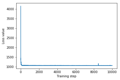
plt.plot(iaf_loss)
plt.xlabel('Training step')
_ = plt.ylabel('Loss value')

IAF surrogate posterior ELBO: -1065.3663330078125

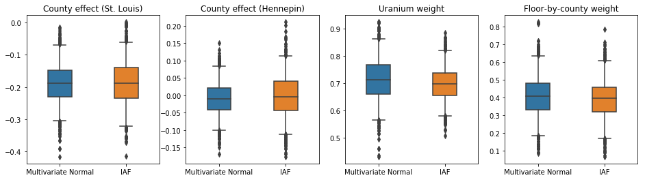
IAF সারোগেট পোস্টেরিয়রের জন্য বিশ্বাসযোগ্য ব্যবধানগুলি সীমাবদ্ধ মাল্টিভেরিয়েট নরমালের মতই দেখা যায়।

results['IAF'] = pack_samples(iaf_samples)
plot_boxplot(results)

বেসলাইন: গড়-ক্ষেত্র সারোগেট পোস্টেরিয়র

VI সারোগেট পোস্টেরিয়রগুলিকে প্রায়শই গড়-ক্ষেত্র (স্বাধীন) সাধারণ বন্টন বলে ধরে নেওয়া হয়, প্রশিক্ষণযোগ্য উপায় এবং ভিন্নতা সহ, যা একটি দ্বিমুখী রূপান্তরের সাথে পূর্বের সমর্থনে সীমাবদ্ধ। আমরা মাল্টিভারিয়েট নরমাল সারোগেট পোস্টেরিয়র হিসাবে একই সাধারণ সূত্র ব্যবহার করে আরও দুটি অভিব্যক্তিপূর্ণ সারোগেট পোস্টেরিয়র ছাড়াও একটি গড়-ক্ষেত্র সারোগেট পোস্টেরিয়র সংজ্ঞায়িত করি।

# A block-diagonal linear operator, in which each block is a diagonal operator,
# transforms the standard Normal base distribution to produce a mean-field
# surrogate posterior.
operators = (tf.linalg.LinearOperatorDiag,
             tf.linalg.LinearOperatorDiag,
             tf.linalg.LinearOperatorDiag)
block_diag_linop = (
    tfp.experimental.vi.util.build_trainable_linear_operator_block(
        operators, flat_event_size))
mean_field_scale = tfb.ScaleMatvecLinearOperatorBlock(block_diag_linop)

mean_field_loc = tfb.JointMap(
    tf.nest.map_structure(
        lambda s: tfb.Shift(
            tf.Variable(tf.random.uniform(
                (s,), minval=-2., maxval=2., dtype=tf.float32))),
        flat_event_size))

mean_field_surrogate_posterior = tfd.TransformedDistribution(
    base_standard_dist,
    bijector = tfb.Chain(  # Note that the chained bijectors are applied in reverse order
        [
         event_space_bijector,  # constrain the surrogate to the support of the prior
         unflatten_bijector,  # pack the reshaped components into the `event_shape` structure of the posterior
         reshape_bijector, # reshape the vector-valued components to match the shapes of the posterior components
         mean_field_loc,   # allow for nonzero mean
         mean_field_scale  # apply the block matrix transformation to the standard Normal distribution
         ]))

optimizer=tf.optimizers.Adam(learning_rate=1e-2)
mean_field_loss = tfp.vi.fit_surrogate_posterior(
    target_model.unnormalized_log_prob,
    mean_field_surrogate_posterior,
    optimizer=optimizer,
    num_steps=10**4,
    sample_size=16,
    jit_compile=True)

mean_field_samples = mean_field_surrogate_posterior.sample(1000)
mean_field_final_elbo = tf.reduce_mean(
    target_model.unnormalized_log_prob(*mean_field_samples)
    - mean_field_surrogate_posterior.log_prob(mean_field_samples))
print('Mean-field surrogate posterior ELBO: {}'.format(mean_field_final_elbo))

plt.plot(mean_field_loss)
plt.xlabel('Training step')
_ = plt.ylabel('Loss value')

Mean-field surrogate posterior ELBO: -1065.7652587890625

এই ক্ষেত্রে, গড় ফিল্ড সারোগেট পোস্টেরিয়র আরও অভিব্যক্তিপূর্ণ সারোগেট পোস্টেরিয়ারের অনুরূপ ফলাফল দেয়, ইঙ্গিত করে যে এই সহজ মডেলটি অনুমান কার্যের জন্য পর্যাপ্ত হতে পারে।

results['Mean Field'] = pack_samples(mean_field_samples)
plot_boxplot(results)

গ্রাউন্ড ট্রুথ: হ্যামিলটোনিয়ান মন্টে কার্লো (HMC)

সারোগেট পোস্টেরিয়ার ফলাফলের সাথে তুলনা করার জন্য আমরা সত্য উত্তর থেকে "গ্রাউন্ড ট্রুথ" নমুনা তৈরি করতে HMC ব্যবহার করি।

num_chains = 8
num_leapfrog_steps = 3
step_size = 0.4
num_steps=20000

flat_event_shape = tf.nest.flatten(target_model.event_shape)
enum_components = list(range(len(flat_event_shape)))
bijector = tfb.Restructure(
    enum_components,
    tf.nest.pack_sequence_as(target_model.event_shape, enum_components))(
        target_model.experimental_default_event_space_bijector())

current_state = bijector(
    tf.nest.map_structure(
        lambda e: tf.zeros([num_chains] + list(e), dtype=tf.float32),
    target_model.event_shape))

hmc = tfp.mcmc.HamiltonianMonteCarlo(
    target_log_prob_fn=target_model.unnormalized_log_prob,
    num_leapfrog_steps=num_leapfrog_steps,
    step_size=[tf.fill(s.shape, step_size) for s in current_state])

hmc = tfp.mcmc.TransformedTransitionKernel(
    hmc, bijector)
hmc = tfp.mcmc.DualAveragingStepSizeAdaptation(
    hmc,
    num_adaptation_steps=int(num_steps // 2 * 0.8),
    target_accept_prob=0.9)

chain, is_accepted = tf.function(
    lambda current_state: tfp.mcmc.sample_chain(
        current_state=current_state,
        kernel=hmc,
        num_results=num_steps // 2,
        num_burnin_steps=num_steps // 2,
        trace_fn=lambda _, pkr:
        (pkr.inner_results.inner_results.is_accepted),
        ),
    autograph=False,
    jit_compile=True)(current_state)

accept_rate = tf.reduce_mean(tf.cast(is_accepted, tf.float32))
ess = tf.nest.map_structure(
    lambda c: tfp.mcmc.effective_sample_size(
        c,
        cross_chain_dims=1,
        filter_beyond_positive_pairs=True),
    chain)

r_hat = tf.nest.map_structure(tfp.mcmc.potential_scale_reduction, chain)
hmc_samples = pack_samples(
    tf.nest.pack_sequence_as(target_model.event_shape, chain))
print('Acceptance rate is {}'.format(accept_rate))

Acceptance rate is 0.9008625149726868

স্যানিটি-চেক HMC ফলাফল প্লট নমুনা ট্রেস.

def plot_traces(var_name, samples):
  fig, axes = plt.subplots(1, 2, figsize=(14, 1.5), sharex='col', sharey='col')
  for chain in range(num_chains):
    s = samples.numpy()[:, chain]
    axes[0].plot(s, alpha=0.7)
    sns.kdeplot(s, ax=axes[1], shade=False)
    axes[0].title.set_text("'{}' trace".format(var_name))
    axes[1].title.set_text("'{}' distribution".format(var_name))
    axes[0].set_xlabel('Iteration')

warnings.filterwarnings('ignore')
for var, var_samples in hmc_samples.items():
  plot_traces(var, var_samples)

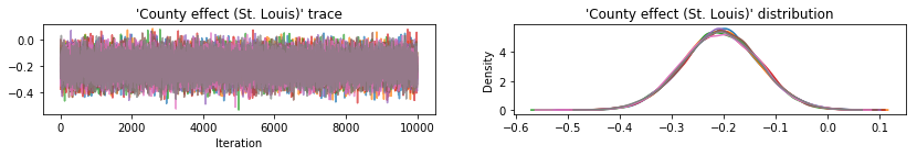
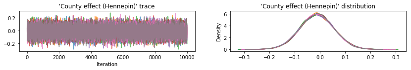
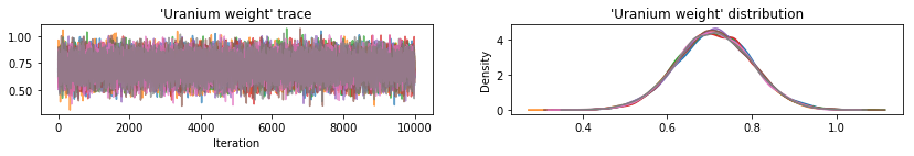
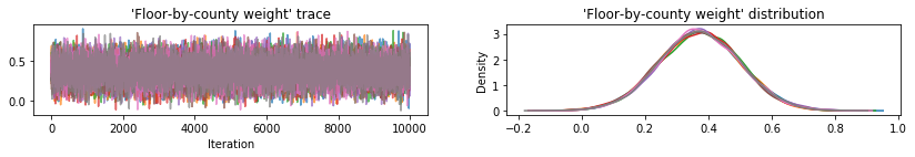
তিনটি সারোগেট পোস্টেরিয়রই বিশ্বাসযোগ্য ব্যবধান তৈরি করেছে যা দৃশ্যত HMC নমুনার মতো, যদিও কখনও কখনও ELBO ক্ষতির প্রভাবের কারণে কম-বিচ্ছুরিত হয়, যেমনটি VI-তে সাধারণ।

results['HMC'] = hmc_samples
plot_boxplot(results)

অতিরিক্ত ফলাফল

প্লটিং ফাংশন

plt.rcParams.update({'axes.titlesize': 'medium', 'xtick.labelsize': 'medium'})
def plot_loss_and_elbo():
  fig, axes = plt.subplots(1, 2, figsize=(12, 4))

  axes[0].scatter([0, 1, 2],
                  [mvn_final_elbo.numpy(),
                  iaf_final_elbo.numpy(),
                  mean_field_final_elbo.numpy()])
  axes[0].set_xticks(ticks=[0, 1, 2])
  axes[0].set_xticklabels(labels=[
    'Multivariate Normal', 'IAF', 'Mean Field'])
  axes[0].title.set_text('Evidence Lower Bound (ELBO)')

  axes[1].plot(mvn_loss, label='Multivariate Normal')
  axes[1].plot(iaf_loss, label='IAF')
  axes[1].plot(mean_field_loss, label='Mean Field')
  axes[1].set_ylim([1000, 4000])
  axes[1].set_xlabel('Training step')
  axes[1].set_ylabel('Loss (negative ELBO)')
  axes[1].title.set_text('Loss')
  plt.legend()
  plt.show()

plt.rcParams.update({'axes.titlesize': 'medium', 'xtick.labelsize': 'small'})
def plot_kdes(num_chains=8):
  fig, axes = plt.subplots(2, 2, figsize=(12, 8))
  k = list(results.values())[0].keys()
  plot_results = {
      v: {p: results[p][v] for p in results} for v in k}
  for i, (var, var_results) in enumerate(plot_results.items()):
    ax = axes[i % 2, i // 2]
    for posterior, posterior_results in var_results.items():
      if posterior == 'HMC':
        label = posterior
        for chain in range(num_chains):
          sns.kdeplot(
              posterior_results[:, chain],
              ax=ax, shade=False, color='k', linestyle=':', label=label)
          label=None
      else:
        sns.kdeplot(
            posterior_results, ax=ax, shade=False, label=posterior)
        ax.title.set_text('{}'.format(var))
    ax.legend()

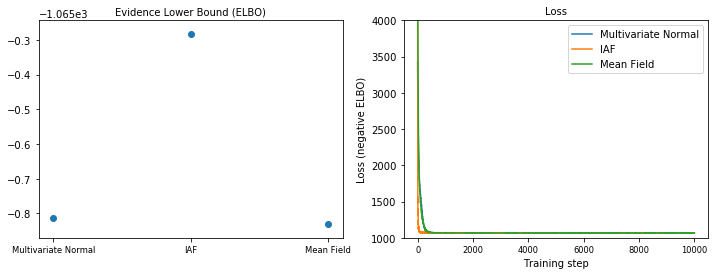
এভিডেন্স লোয়ার বাউন্ড (ELBO)

IAF, এখন পর্যন্ত সবচেয়ে বড় এবং সবচেয়ে নমনীয় সারোগেট পোস্টেরিয়র, সর্বোচ্চ এভিডেন্স লোয়ার বাউন্ডে (ELBO) রূপান্তরিত হয়।

plot_loss_and_elbo()

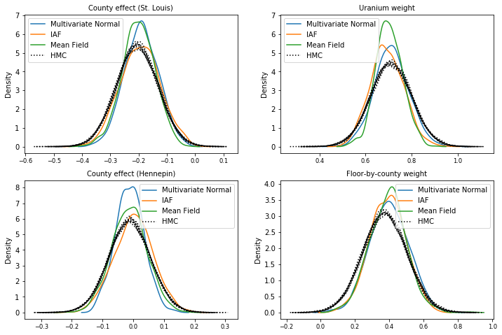
পরবর্তী নমুনা

এইচএমসি গ্রাউন্ড ট্রুথ নমুনার সাথে তুলনা করে প্রতিটি সারোগেট পোস্টেরিয়র থেকে নমুনা (বক্স প্লটে দেখানো নমুনার একটি ভিন্ন ভিজ্যুয়ালাইজেশন)।

plot_kdes()

উপসংহার

এই Colab-এ, আমরা জয়েন্ট ডিস্ট্রিবিউশন এবং মাল্টিপার্ট বাইজেক্টর ব্যবহার করে VI সারোগেট পোস্টেরিয়র তৈরি করেছি এবং রেডন ডেটাসেটে রিগ্রেশন মডেলে ওজনের জন্য বিশ্বাসযোগ্য ব্যবধান অনুমান করার জন্য সেগুলিকে ফিট করেছি। এই সাধারণ মডেলের জন্য, আরও অভিব্যক্তিপূর্ণ সারোগেট পোস্টেরিয়রগুলি একটি গড়-ক্ষেত্র সারোগেট পোস্টেরিয়রের অনুরূপভাবে সঞ্চালিত হয়। আমরা যে সরঞ্জামগুলি প্রদর্শন করেছি, তবে, আরও জটিল মডেলগুলির জন্য উপযুক্ত নমনীয় সারোগেট পোস্টেরিয়ারগুলির বিস্তৃত পরিসর তৈরি করতে ব্যবহার করা যেতে পারে।