
| | |  عرض المصدر على جيثب عرض المصدر على جيثب | |
يستكشف هذا البرنامج التعليمي خوارزميات حساب التدرج لقيم توقع دوائر الكم.
يعد حساب التدرج اللوني لقيمة توقع معينة يمكن ملاحظتها في دائرة كمومية عملية متضمنة. لا تتمتع القيم المتوقعة للملاحظات برفاهية وجود صيغ تدرج تحليلي يسهل دائمًا تدوينها - على عكس تحويلات التعلم الآلي التقليدية مثل مضاعفة المصفوفة أو إضافة المتجه التي تحتوي على صيغ تدرج تحليلي يسهل تدوينها. نتيجة لذلك ، هناك طرق مختلفة لحساب التدرج الكمي مفيدة لسيناريوهات مختلفة. يقارن هذا البرنامج التعليمي ويقارن بين مخططين مختلفين للتمايز.
يثبت
pip install tensorflow==2.7.0
تثبيت TensorFlow Quantum:
pip install tensorflow-quantum
# Update package resources to account for version changes.
import importlib, pkg_resources
importlib.reload(pkg_resources)
<module 'pkg_resources' from '/tmpfs/src/tf_docs_env/lib/python3.7/site-packages/pkg_resources/__init__.py'>
الآن قم باستيراد TensorFlow وتبعيات الوحدة النمطية:
import tensorflow as tf
import tensorflow_quantum as tfq

import cirq
import sympy
import numpy as np

# visualization tools
%matplotlib inline
import matplotlib.pyplot as plt
from cirq.contrib.svg import SVGCircuit
2022-02-04 12:25:24.733670: E tensorflow/stream_executor/cuda/cuda_driver.cc:271] failed call to cuInit: CUDA_ERROR_NO_DEVICE: no CUDA-capable device is detected
1. تمهيدية
دعونا نجعل فكرة حساب التدرج لدارات الكم أكثر واقعية. افترض أن لديك دائرة ذات معلمات مثل هذه:
qubit = cirq.GridQubit(0, 0)
my_circuit = cirq.Circuit(cirq.Y(qubit)**sympy.Symbol('alpha'))
SVGCircuit(my_circuit)
findfont: Font family ['Arial'] not found. Falling back to DejaVu Sans.

جنبًا إلى جنب مع:
pauli_x = cirq.X(qubit)
pauli_x
cirq.X(cirq.GridQubit(0, 0))
بالنظر إلى عامل التشغيل هذا ، فأنت تعلم أن \(⟨Y(\alpha)| X | Y(\alpha)⟩ = \sin(\pi \alpha)\)
def my_expectation(op, alpha):
    """Compute ⟨Y(alpha)| `op` | Y(alpha)⟩"""
    params = {'alpha': alpha}
    sim = cirq.Simulator()
    final_state_vector = sim.simulate(my_circuit, params).final_state_vector
    return op.expectation_from_state_vector(final_state_vector, {qubit: 0}).real


my_alpha = 0.3
print("Expectation=", my_expectation(pauli_x, my_alpha))
print("Sin Formula=", np.sin(np.pi * my_alpha))
Expectation= 0.80901700258255
Sin Formula= 0.8090169943749475
وإذا قمت بتعريف \(f_{1}(\alpha) = ⟨Y(\alpha)| X | Y(\alpha)⟩\) ثم \(f_{1}^{'}(\alpha) = \pi \cos(\pi \alpha)\). دعنا نتحقق من هذا:
def my_grad(obs, alpha, eps=0.01):
    grad = 0
    f_x = my_expectation(obs, alpha)
    f_x_prime = my_expectation(obs, alpha + eps)
    return ((f_x_prime - f_x) / eps).real


print('Finite difference:', my_grad(pauli_x, my_alpha))
print('Cosine formula:   ', np.pi * np.cos(np.pi * my_alpha))
Finite difference: 1.8063604831695557
Cosine formula:    1.8465818304904567
2. الحاجة إلى أداة تفاضل
مع الدوائر الأكبر ، لن تكون دائمًا محظوظًا جدًا لامتلاك صيغة تحسب بدقة التدرجات اللونية لدائرة كمومية معينة. في حالة عدم كفاية الصيغة البسيطة لحساب التدرج اللوني ، تسمح لك فئة tfq.differentiators.Differentiator بتعريف الخوارزميات لحساب تدرجات دوائرك. على سبيل المثال ، يمكنك إعادة إنشاء المثال أعلاه في TensorFlow Quantum (TFQ) باستخدام:
expectation_calculation = tfq.layers.Expectation(
    differentiator=tfq.differentiators.ForwardDifference(grid_spacing=0.01))

expectation_calculation(my_circuit,
                        operators=pauli_x,
                        symbol_names=['alpha'],
                        symbol_values=[[my_alpha]])
<tf.Tensor: shape=(1, 1), dtype=float32, numpy=array([[0.80901706]], dtype=float32)>
ومع ذلك ، إذا قمت بالتبديل إلى تقدير التوقعات بناءً على أخذ العينات (ما قد يحدث على جهاز حقيقي) ، يمكن أن تتغير القيم قليلاً. هذا يعني أنه لديك الآن تقدير غير كامل:
sampled_expectation_calculation = tfq.layers.SampledExpectation(
    differentiator=tfq.differentiators.ForwardDifference(grid_spacing=0.01))

sampled_expectation_calculation(my_circuit,
                                operators=pauli_x,
                                repetitions=500,
                                symbol_names=['alpha'],
                                symbol_values=[[my_alpha]])
<tf.Tensor: shape=(1, 1), dtype=float32, numpy=array([[0.836]], dtype=float32)>
يمكن أن يتطور هذا بسرعة إلى مشكلة دقة خطيرة عندما يتعلق الأمر بالتدرجات:
# Make input_points = [batch_size, 1] array.
input_points = np.linspace(0, 5, 200)[:, np.newaxis].astype(np.float32)
exact_outputs = expectation_calculation(my_circuit,
operators=pauli_x,
symbol_names=['alpha'],
symbol_values=input_points)
imperfect_outputs = sampled_expectation_calculation(my_circuit,
operators=pauli_x,
repetitions=500,
symbol_names=['alpha'],
symbol_values=input_points)
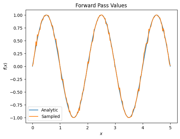
plt.title('Forward Pass Values')
plt.xlabel('$x$')
plt.ylabel('$f(x)$')
plt.plot(input_points, exact_outputs, label='Analytic')
plt.plot(input_points, imperfect_outputs, label='Sampled')
plt.legend()
<matplotlib.legend.Legend at 0x7ff07d556190>
# Gradients are a much different story.
values_tensor = tf.convert_to_tensor(input_points)

with tf.GradientTape() as g:
    g.watch(values_tensor)
    exact_outputs = expectation_calculation(my_circuit,
                                            operators=pauli_x,
                                            symbol_names=['alpha'],
                                            symbol_values=values_tensor)
analytic_finite_diff_gradients = g.gradient(exact_outputs, values_tensor)

with tf.GradientTape() as g:
    g.watch(values_tensor)
    imperfect_outputs = sampled_expectation_calculation(
        my_circuit,
        operators=pauli_x,
        repetitions=500,
        symbol_names=['alpha'],
        symbol_values=values_tensor)
sampled_finite_diff_gradients = g.gradient(imperfect_outputs, values_tensor)

plt.title('Gradient Values')
plt.xlabel('$x$')
plt.ylabel('$f^{\'}(x)$')
plt.plot(input_points, analytic_finite_diff_gradients, label='Analytic')
plt.plot(input_points, sampled_finite_diff_gradients, label='Sampled')
plt.legend()
<matplotlib.legend.Legend at 0x7ff07adb8dd0>
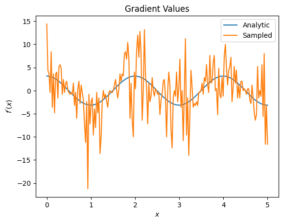
هنا يمكنك أن ترى أنه على الرغم من أن صيغة الفروق المحدودة سريعة في حساب التدرجات نفسها في الحالة التحليلية ، عندما يتعلق الأمر بالطرق القائمة على أخذ العينات ، فقد كانت صاخبة جدًا. يجب استخدام تقنيات أكثر دقة لضمان إمكانية حساب التدرج اللوني الجيد. بعد ذلك ، سوف تنظر إلى تقنية أبطأ بكثير والتي لن تكون مناسبة تمامًا لحسابات التدرج التوقع التحليلي ، ولكنها تؤدي أداءً أفضل بكثير في الحالة القائمة على العينة في العالم الحقيقي:
# A smarter differentiation scheme.
gradient_safe_sampled_expectation = tfq.layers.SampledExpectation(
    differentiator=tfq.differentiators.ParameterShift())

with tf.GradientTape() as g:
    g.watch(values_tensor)
    imperfect_outputs = gradient_safe_sampled_expectation(
        my_circuit,
        operators=pauli_x,
        repetitions=500,
        symbol_names=['alpha'],
        symbol_values=values_tensor)

sampled_param_shift_gradients = g.gradient(imperfect_outputs, values_tensor)

plt.title('Gradient Values')
plt.xlabel('$x$')
plt.ylabel('$f^{\'}(x)$')
plt.plot(input_points, analytic_finite_diff_gradients, label='Analytic')
plt.plot(input_points, sampled_param_shift_gradients, label='Sampled')
plt.legend()
<matplotlib.legend.Legend at 0x7ff07ad9ff90>
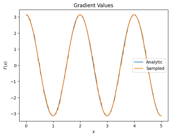
مما سبق ، يمكنك أن ترى أنه من الأفضل استخدام أدوات تفاضل معينة لسيناريوهات بحث معينة. بشكل عام ، تعتبر الطرق الأبطأ القائمة على العينات والتي تكون قوية ضد ضوضاء الجهاز ، وما إلى ذلك ، عوامل تفاضل كبيرة عند اختبار أو تنفيذ الخوارزميات في إعداد "عالم أكثر واقعية". تعتبر الطرق الأسرع مثل الفروق المحدودة رائعة بالنسبة للحسابات التحليلية وتريد إنتاجية أعلى ، لكنك لا تهتم بعد بصلاحية الجهاز في الخوارزمية الخاصة بك.
3. مراقبات متعددة
دعنا نقدم ثانية يمكن ملاحظتها ونرى كيف يدعم TensorFlow Quantum العديد من الملاحظات لدائرة واحدة.
pauli_z = cirq.Z(qubit)
pauli_z
cirq.Z(cirq.GridQubit(0, 0))
إذا تم استخدام هذه الملاحظة مع نفس الدائرة كما كان من قبل ، فسيكون لديك \(f_{2}(\alpha) = ⟨Y(\alpha)| Z | Y(\alpha)⟩ = \cos(\pi \alpha)\) و \(f_{2}^{'}(\alpha) = -\pi \sin(\pi \alpha)\). قم بإجراء فحص سريع:
test_value = 0.

print('Finite difference:', my_grad(pauli_z, test_value))
print('Sin formula:      ', -np.pi * np.sin(np.pi * test_value))
Finite difference: -0.04934072494506836
Sin formula:       -0.0
إنها مباراة (قريبة بما فيه الكفاية).
الآن إذا \(g(\alpha) = f_{1}(\alpha) + f_{2}(\alpha)\) ثم \(g'(\alpha) = f_{1}^{'}(\alpha) + f^{'}_{2}(\alpha)\). تحديد أكثر من واحد يمكن ملاحظته في TensorFlow Quantum لاستخدامه مع دائرة ما يعادل إضافة المزيد من المصطلحات إلى \(g\).
هذا يعني أن التدرج اللوني لرمز معين في دائرة ما يساوي مجموع التدرجات فيما يتعلق بكل ما يمكن ملاحظته لهذا الرمز المطبق على تلك الدائرة. هذا متوافق مع أخذ التدرج اللوني TensorFlow و backpropagation (حيث تعطي مجموع التدرجات على جميع الملحوظات كتدرج لرمز معين).
sum_of_outputs = tfq.layers.Expectation(
    differentiator=tfq.differentiators.ForwardDifference(grid_spacing=0.01))

sum_of_outputs(my_circuit,
               operators=[pauli_x, pauli_z],
               symbol_names=['alpha'],
               symbol_values=[[test_value]])
<tf.Tensor: shape=(1, 2), dtype=float32, numpy=array([[1.9106855e-15, 1.0000000e+00]], dtype=float32)>
هنا ترى المدخل الأول هو التوقع wrt Pauli X ، والثاني هو التوقع wrt Pauli Z. الآن عندما تأخذ التدرج:
test_value_tensor = tf.convert_to_tensor([[test_value]])

with tf.GradientTape() as g:
    g.watch(test_value_tensor)
    outputs = sum_of_outputs(my_circuit,
                             operators=[pauli_x, pauli_z],
                             symbol_names=['alpha'],
                             symbol_values=test_value_tensor)

sum_of_gradients = g.gradient(outputs, test_value_tensor)

print(my_grad(pauli_x, test_value) + my_grad(pauli_z, test_value))
print(sum_of_gradients.numpy())
3.0917350202798843
[[3.0917213]]
لقد تحققت هنا من أن مجموع التدرجات لكل ما يمكن ملاحظته هو بالفعل تدرج \(\alpha\). يتم دعم هذا السلوك من قبل جميع تفاضلات TensorFlow Quantum ويلعب دورًا مهمًا في التوافق مع باقي TensorFlow.
4. الاستخدام المتقدم
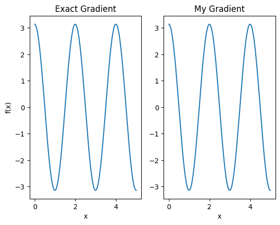
جميع التفاضلات الموجودة داخل TensorFlow Quantum subclass tfq.differentiators.Differentiator . لتنفيذ أداة التمييز ، يجب على المستخدم تنفيذ واحدة من واجهتين. المعيار هو تنفيذ get_gradient_circuits ، والذي يخبر الفئة الأساسية بالدوائر التي يجب قياسها للحصول على تقدير للتدرج. بدلاً من ذلك ، يمكنك زيادة التحميل على differentiate_analytic و differentiate_sampled ؛ الفصل tfq.differentiators.Adjoint يأخذ هذا الطريق.
يستخدم ما يلي TensorFlow Quantum لتنفيذ التدرج اللوني للدائرة. ستستخدم مثالًا صغيرًا لتغيير المعلمات.
استدع الدائرة التي حددتها أعلاه ، \(|\alpha⟩ = Y^{\alpha}|0⟩\). كما كان من قبل ، يمكنك تحديد وظيفة على أنها القيمة المتوقعة لهذه الدائرة مقابل \(X\) يمكن ملاحظته ، \(f(\alpha) = ⟨\alpha|X|\alpha⟩\). باستخدام قواعد إزاحة المعلمات ، في هذه الدائرة ، يمكنك معرفة أن المشتق هو
\[\frac{\partial}{\partial \alpha} f(\alpha) = \frac{\pi}{2} f\left(\alpha + \frac{1}{2}\right) - \frac{ \pi}{2} f\left(\alpha - \frac{1}{2}\right)\]
ترجع الدالة get_gradient_circuits مكونات هذا المشتق.
class MyDifferentiator(tfq.differentiators.Differentiator):
    """A Toy differentiator for <Y^alpha | X |Y^alpha>."""

    def __init__(self):
        pass

    def get_gradient_circuits(self, programs, symbol_names, symbol_values):
        """Return circuits to compute gradients for given forward pass circuits.

        Every gradient on a quantum computer can be computed via measurements
        of transformed quantum circuits.  Here, you implement a custom gradient
        for a specific circuit.  For a real differentiator, you will need to
        implement this function in a more general way.  See the differentiator
        implementations in the TFQ library for examples.
        """

        # The two terms in the derivative are the same circuit...
        batch_programs = tf.stack([programs, programs], axis=1)

        # ... with shifted parameter values.
        shift = tf.constant(1/2)
        forward = symbol_values + shift
        backward = symbol_values - shift
        batch_symbol_values = tf.stack([forward, backward], axis=1)

        # Weights are the coefficients of the terms in the derivative.
        num_program_copies = tf.shape(batch_programs)[0]
        batch_weights = tf.tile(tf.constant([[[np.pi/2, -np.pi/2]]]),
                                [num_program_copies, 1, 1])

        # The index map simply says which weights go with which circuits.
        batch_mapper = tf.tile(
            tf.constant([[[0, 1]]]), [num_program_copies, 1, 1])

        return (batch_programs, symbol_names, batch_symbol_values,
                batch_weights, batch_mapper)
تستخدم فئة Differentiator الأساسية المكونات التي تم إرجاعها من get_gradient_circuits لحساب المشتق ، كما هو الحال في صيغة تغيير المعلمة التي رأيتها أعلاه. يمكن الآن استخدام أداة التمييز الجديدة هذه مع كائنات tfq.layer الموجودة:
custom_dif = MyDifferentiator()
custom_grad_expectation = tfq.layers.Expectation(differentiator=custom_dif)

# Now let's get the gradients with finite diff.
with tf.GradientTape() as g:
    g.watch(values_tensor)
    exact_outputs = expectation_calculation(my_circuit,
                                            operators=[pauli_x],
                                            symbol_names=['alpha'],
                                            symbol_values=values_tensor)

analytic_finite_diff_gradients = g.gradient(exact_outputs, values_tensor)

# Now let's get the gradients with custom diff.
with tf.GradientTape() as g:
    g.watch(values_tensor)
    my_outputs = custom_grad_expectation(my_circuit,
                                         operators=[pauli_x],
                                         symbol_names=['alpha'],
                                         symbol_values=values_tensor)

my_gradients = g.gradient(my_outputs, values_tensor)

plt.subplot(1, 2, 1)
plt.title('Exact Gradient')
plt.plot(input_points, analytic_finite_diff_gradients.numpy())
plt.xlabel('x')
plt.ylabel('f(x)')
plt.subplot(1, 2, 2)
plt.title('My Gradient')
plt.plot(input_points, my_gradients.numpy())
plt.xlabel('x')
Text(0.5, 0, 'x')
يمكن الآن استخدام أداة التفاضل الجديدة هذه لإنشاء عمليات قابلة للتفاضل.
# Create a noisy sample based expectation op.
expectation_sampled = tfq.get_sampled_expectation_op(
    cirq.DensityMatrixSimulator(noise=cirq.depolarize(0.01)))

# Make it differentiable with your differentiator:
# Remember to refresh the differentiator before attaching the new op
custom_dif.refresh()
differentiable_op = custom_dif.generate_differentiable_op(
    sampled_op=expectation_sampled)

# Prep op inputs.
circuit_tensor = tfq.convert_to_tensor([my_circuit])
op_tensor = tfq.convert_to_tensor([[pauli_x]])
single_value = tf.convert_to_tensor([[my_alpha]])
num_samples_tensor = tf.convert_to_tensor([[5000]])

with tf.GradientTape() as g:
    g.watch(single_value)
    forward_output = differentiable_op(circuit_tensor, ['alpha'], single_value,
                                       op_tensor, num_samples_tensor)

my_gradients = g.gradient(forward_output, single_value)

print('---TFQ---')
print('Foward:  ', forward_output.numpy())
print('Gradient:', my_gradients.numpy())
print('---Original---')
print('Forward: ', my_expectation(pauli_x, my_alpha))
print('Gradient:', my_grad(pauli_x, my_alpha))
---TFQ---
Foward:   [[0.8016]]
Gradient: [[1.7932211]]
---Original---
Forward:  0.80901700258255
Gradient: 1.8063604831695557