TensorFlow 14 মে Google I/O-তে ফিরে এসেছে! এখন নিবন্ধন করুন

এই পৃষ্ঠাটি Cloud Translation API অনুবাদ করেছে।

কোয়ান্টাম কনভোল্যুশনাল নিউরাল নেটওয়ার্ক

TensorFlow.org-এ দেখুন

Google Colab-এ চালান

GitHub-এ উৎস দেখুন

নোটবুক ডাউনলোড করুন

এই টিউটোরিয়ালটি একটি সরলীকৃত কোয়ান্টাম কনভোলিউশনাল নিউরাল নেটওয়ার্ক (QCNN) প্রয়োগ করে, একটি প্রস্তাবিত কোয়ান্টাম অ্যানালগ যা একটি ক্লাসিক্যাল কনভোলিউশনাল নিউরাল নেটওয়ার্ক যা অনুবাদকভাবে অপরিবর্তনীয় ।

এই উদাহরণটি প্রদর্শন করে যে কীভাবে একটি কোয়ান্টাম ডেটা উত্সের নির্দিষ্ট বৈশিষ্ট্যগুলি সনাক্ত করা যায়, যেমন একটি কোয়ান্টাম সেন্সর বা একটি ডিভাইস থেকে একটি জটিল সিমুলেশন। কোয়ান্টাম ডেটা সোর্স একটি ক্লাস্টার স্টেট যেটিতে উত্তেজনা থাকতে পারে বা নাও থাকতে পারে—কি QCNN সনাক্ত করতে শিখবে (কাগজে ব্যবহৃত ডেটাসেটটি SPT ফেজ শ্রেণীবিভাগ ছিল)।

সেটআপ

pip install tensorflow==2.7.0

টেনসরফ্লো কোয়ান্টাম ইনস্টল করুন:

pip install tensorflow-quantum

# Update package resources to account for version changes.
import importlib, pkg_resources
importlib.reload(pkg_resources)

<module 'pkg_resources' from '/tmpfs/src/tf_docs_env/lib/python3.7/site-packages/pkg_resources/__init__.py'>

এখন TensorFlow এবং মডিউল নির্ভরতা আমদানি করুন:

import tensorflow as tf
import tensorflow_quantum as tfq

import cirq
import sympy
import numpy as np

# visualization tools
%matplotlib inline
import matplotlib.pyplot as plt
from cirq.contrib.svg import SVGCircuit

2022-02-04 12:43:45.380301: E tensorflow/stream_executor/cuda/cuda_driver.cc:271] failed call to cuInit: CUDA_ERROR_NO_DEVICE: no CUDA-capable device is detected

1. একটি QCNN তৈরি করুন

1.1 একটি টেনসরফ্লো গ্রাফে সার্কিট একত্রিত করুন

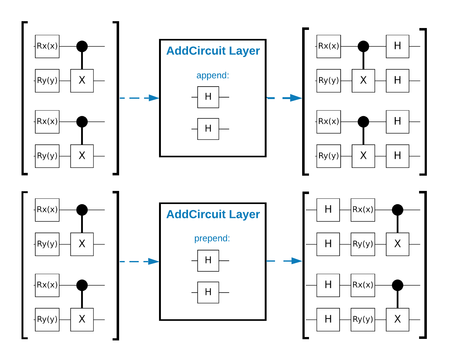
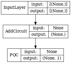
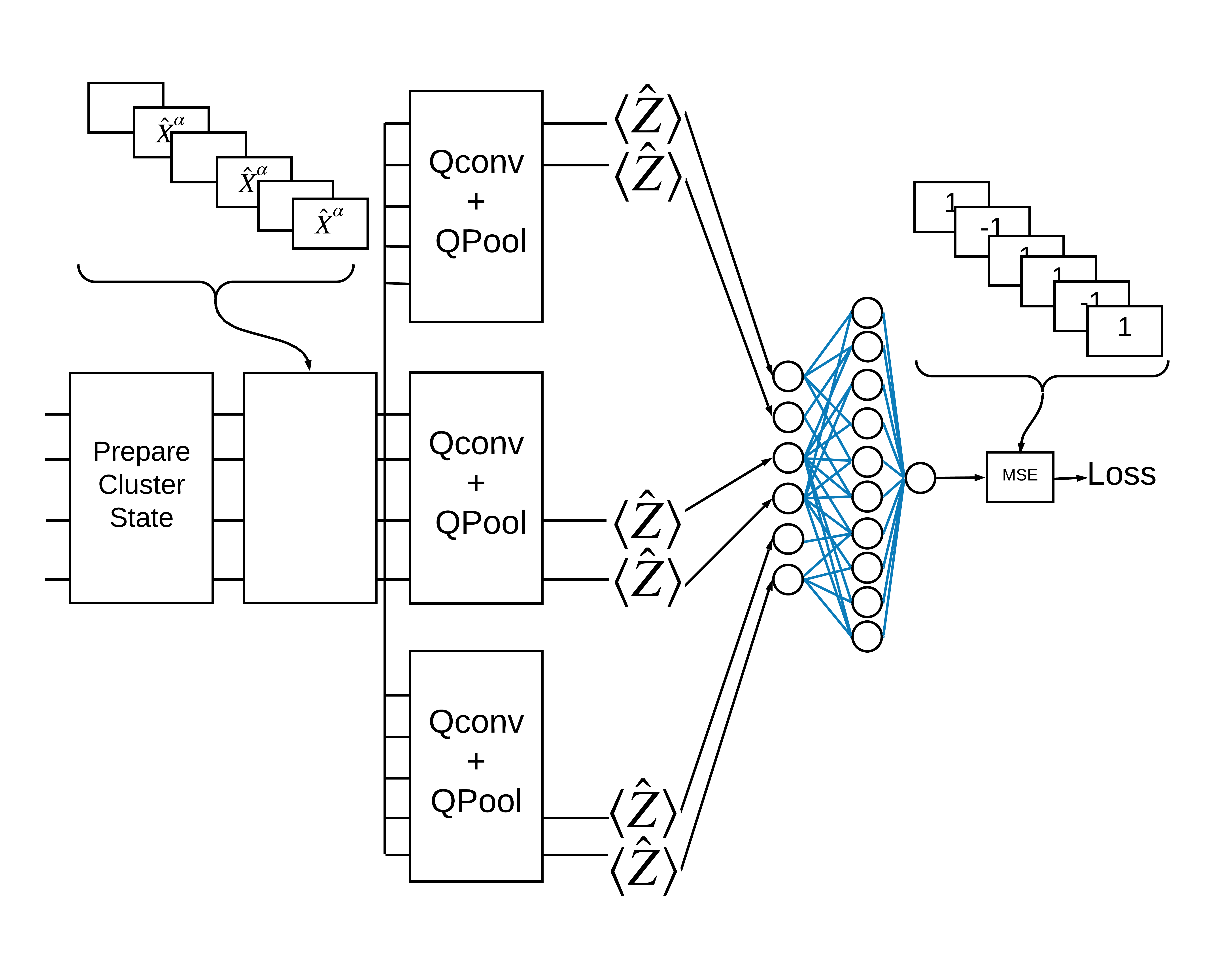
টেনসরফ্লো কোয়ান্টাম (TFQ) ইন-গ্রাফ সার্কিট নির্মাণের জন্য ডিজাইন করা লেয়ার ক্লাস প্রদান করে। একটি উদাহরণ হল tfq.layers.AddCircuit স্তর যা tf.keras.Layer থেকে উত্তরাধিকারসূত্রে পাওয়া যায়। এই লেয়ারটি সার্কিটের ইনপুট ব্যাচে প্রিপেন্ড বা যুক্ত করতে পারে, যেমনটি নিচের চিত্রে দেখানো হয়েছে।

নিম্নলিখিত স্নিপেট এই স্তর ব্যবহার করে:

qubit = cirq.GridQubit(0, 0)

# Define some circuits.
circuit1 = cirq.Circuit(cirq.X(qubit))
circuit2 = cirq.Circuit(cirq.H(qubit))

# Convert to a tensor.
input_circuit_tensor = tfq.convert_to_tensor([circuit1, circuit2])

# Define a circuit that we want to append
y_circuit = cirq.Circuit(cirq.Y(qubit))

# Instantiate our layer
y_appender = tfq.layers.AddCircuit()

# Run our circuit tensor through the layer and save the output.
output_circuit_tensor = y_appender(input_circuit_tensor, append=y_circuit)

ইনপুট টেনসর পরীক্ষা করুন:

print(tfq.from_tensor(input_circuit_tensor))

[cirq.Circuit([
     cirq.Moment(
         cirq.X(cirq.GridQubit(0, 0)),
     ),
 ])
 cirq.Circuit([
     cirq.Moment(
         cirq.H(cirq.GridQubit(0, 0)),
     ),
 ])                                   ]

এবং আউটপুট টেনসর পরীক্ষা করুন:

print(tfq.from_tensor(output_circuit_tensor))

[cirq.Circuit([
     cirq.Moment(
         cirq.X(cirq.GridQubit(0, 0)),
     ),
     cirq.Moment(
         cirq.Y(cirq.GridQubit(0, 0)),
     ),
 ])
 cirq.Circuit([
     cirq.Moment(
         cirq.H(cirq.GridQubit(0, 0)),
     ),
     cirq.Moment(
         cirq.Y(cirq.GridQubit(0, 0)),
     ),
 ])                                   ]

যদিও tfq.layers.AddCircuit ব্যবহার না করে নীচের উদাহরণগুলি চালানো সম্ভব, এটি বোঝার একটি ভাল সুযোগ যে কীভাবে জটিল কার্যকারিতা টেনসরফ্লো কম্পিউট গ্রাফগুলিতে এম্বেড করা যেতে পারে।

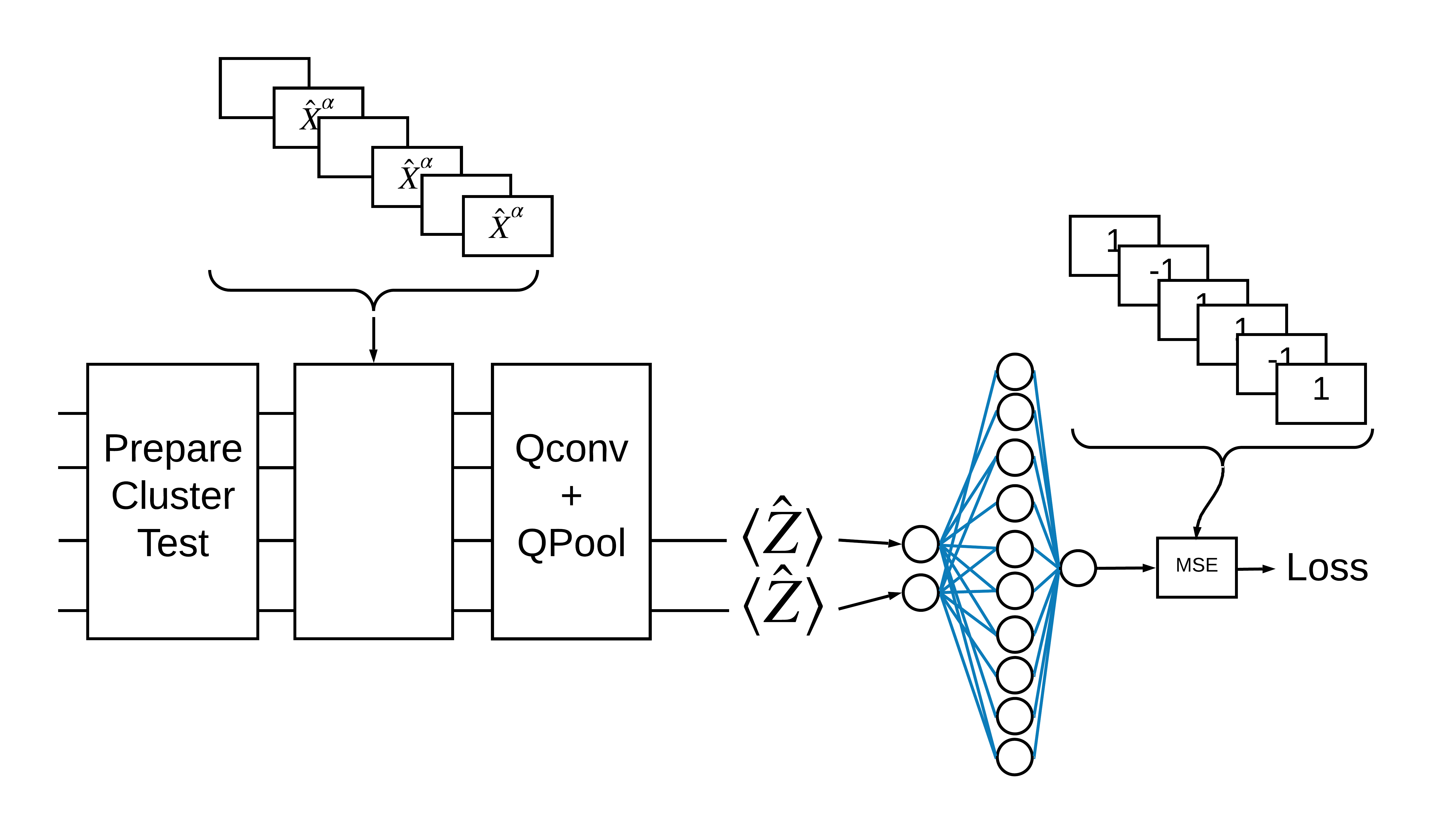
1.2 সমস্যা ওভারভিউ

আপনি একটি ক্লাস্টার স্টেট প্রস্তুত করবেন এবং এটি "উত্তেজিত" কিনা তা সনাক্ত করতে একটি কোয়ান্টাম ক্লাসিফায়ারকে প্রশিক্ষণ দেবেন। ক্লাস্টার স্টেটটি অত্যন্ত জটিল কিন্তু একটি ক্লাসিক্যাল কম্পিউটারের জন্য অগত্যা কঠিন নয়। স্পষ্টতার জন্য, এটি কাগজে ব্যবহৃত ডেটাসেটের চেয়ে সহজ ডেটাসেট।

এই শ্রেণীবিভাগের কাজের জন্য আপনি একটি গভীর MERA- এর মতো QCNN আর্কিটেকচার বাস্তবায়ন করবেন যেহেতু:

QCNN এর মত, একটি রিং এর ক্লাস্টার অবস্থা অনুবাদগতভাবে অপরিবর্তনীয়।
ক্লাস্টার রাষ্ট্র অত্যন্ত জট আছে.

এই স্থাপত্যটি জট কমাতে কার্যকর হওয়া উচিত, একটি একক কিউবিট পড়ার মাধ্যমে শ্রেণীবিভাগ প্রাপ্ত করা।

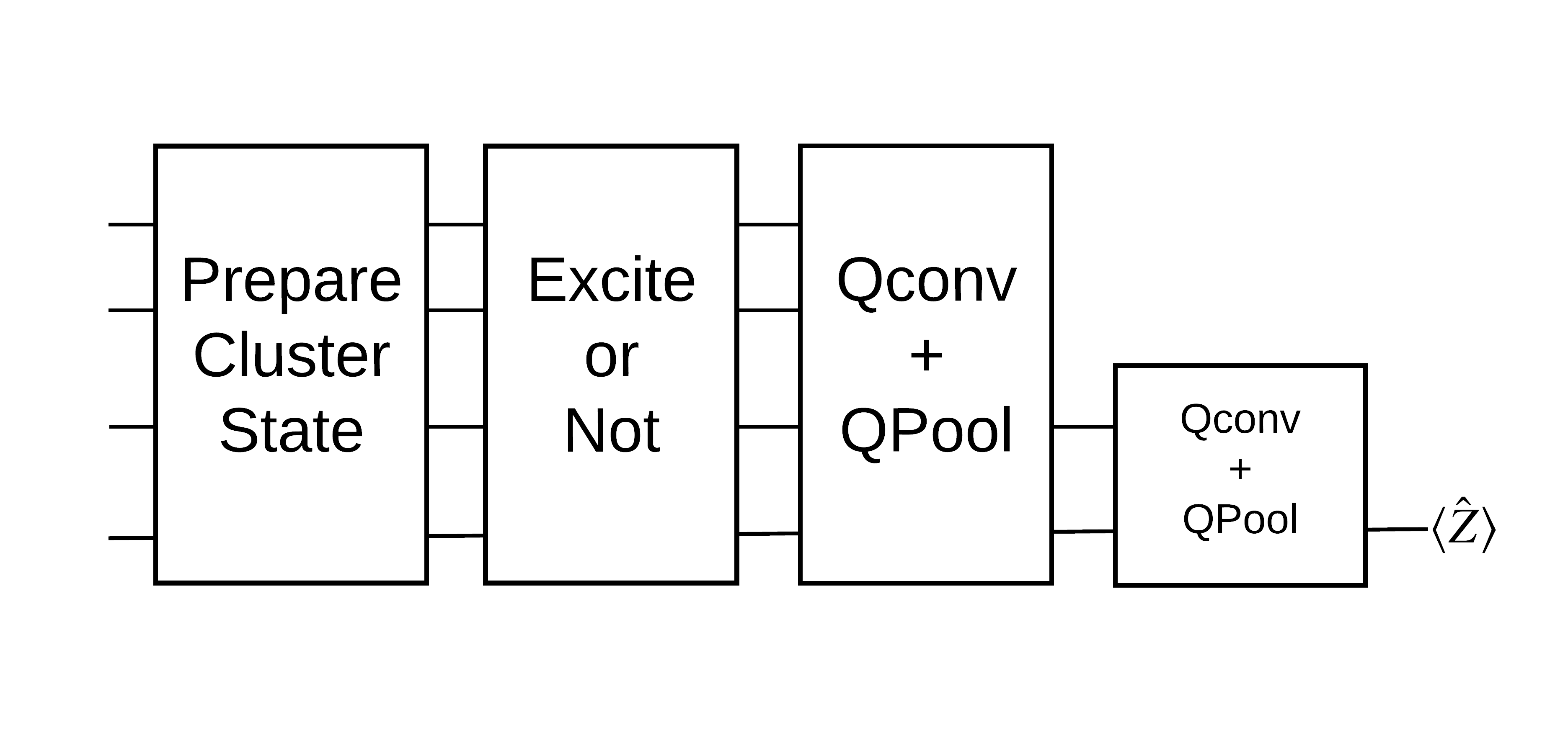
একটি "উত্তেজিত" ক্লাস্টার স্টেটকে একটি ক্লাস্টার স্টেট হিসাবে সংজ্ঞায়িত করা হয় যেটির যেকোনো কিউবিটে একটি cirq.rx গেট প্রয়োগ করা হয়েছে। Qconv এবং QPool এই টিউটোরিয়ালে পরে আলোচনা করা হয়েছে।

1.3 TensorFlow-এর জন্য বিল্ডিং ব্লক

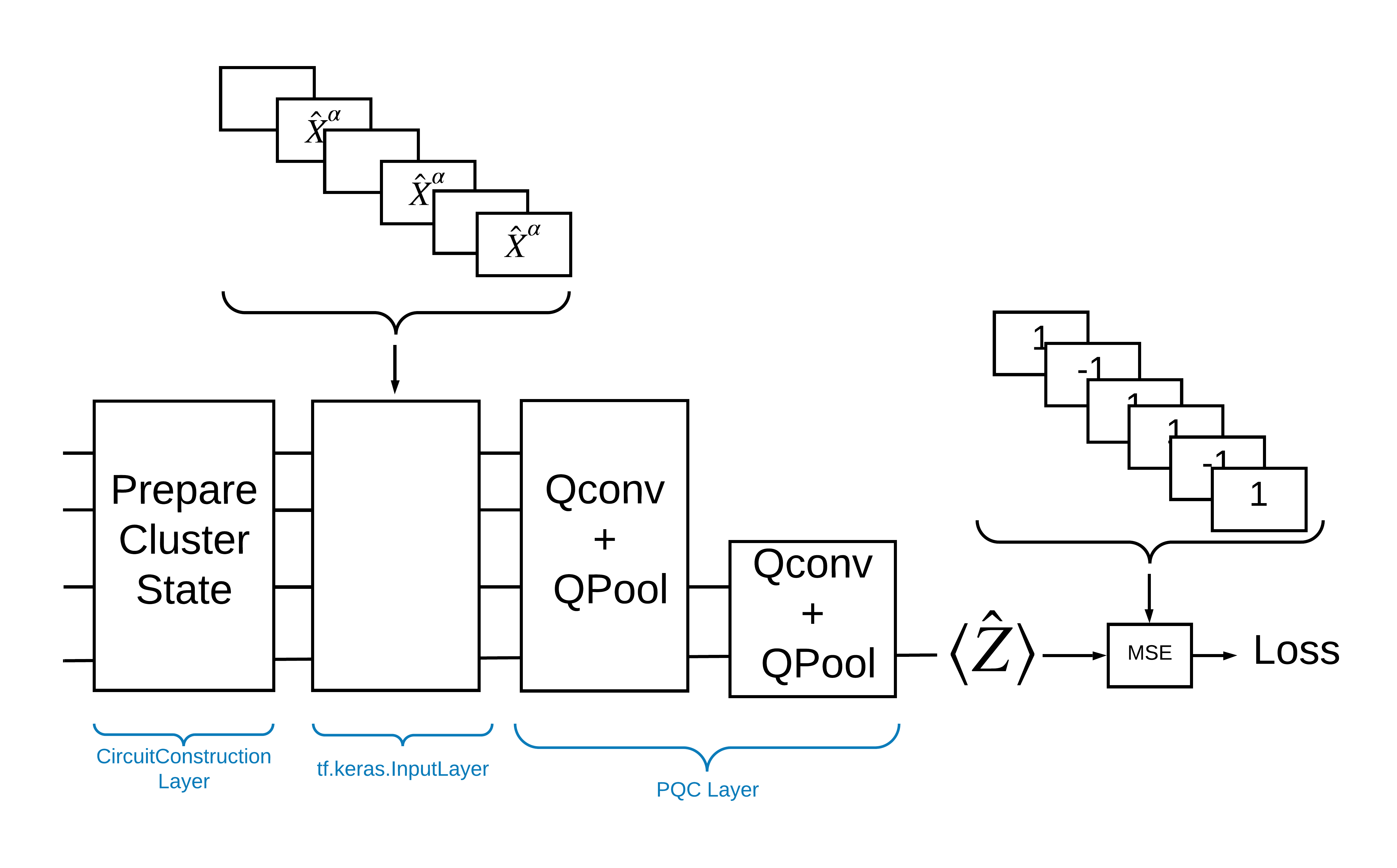
TensorFlow কোয়ান্টামের সাথে এই সমস্যাটি সমাধান করার একটি উপায় হল নিম্নলিখিতগুলি বাস্তবায়ন করা:

মডেলের ইনপুট হল একটি সার্কিট টেনসর—হয় একটি খালি সার্কিট বা একটি এক্স গেট একটি নির্দিষ্ট কিউবিটে উত্তেজনা নির্দেশ করে।
মডেলের বাকি কোয়ান্টাম উপাদানগুলো tfq.layers.AddCircuit লেয়ার দিয়ে তৈরি।
অনুমানের জন্য একটি tfq.layers.PQC স্তর ব্যবহার করা হয়। এটি \(\langle \hat{Z} \rangle\) পড়ে এবং এটি একটি উত্তেজিত অবস্থার জন্য 1 এর লেবেলের সাথে বা একটি অ-উত্তেজিত অবস্থার জন্য -1 এর সাথে তুলনা করে।

1.4 ডেটা

আপনার মডেল তৈরি করার আগে, আপনি আপনার ডেটা তৈরি করতে পারেন। এই ক্ষেত্রে এটি ক্লাস্টার অবস্থায় উত্তেজনা হতে চলেছে (মূল কাগজটি আরও জটিল ডেটাসেট ব্যবহার করে)। উত্তেজনাকে cirq.rx গেট দিয়ে উপস্থাপন করা হয়। যথেষ্ট বড় ঘূর্ণন একটি উত্তেজনা বলে মনে করা হয় এবং 1 লেবেল করা হয় এবং একটি ঘূর্ণন যা যথেষ্ট বড় নয় তাকে -1 লেবেল করা হয় এবং একটি উত্তেজনা নয় বলে মনে করা হয়।

def generate_data(qubits):
    """Generate training and testing data."""
    n_rounds = 20  # Produces n_rounds * n_qubits datapoints.
    excitations = []
    labels = []
    for n in range(n_rounds):
        for bit in qubits:
            rng = np.random.uniform(-np.pi, np.pi)
            excitations.append(cirq.Circuit(cirq.rx(rng)(bit)))
            labels.append(1 if (-np.pi / 2) <= rng <= (np.pi / 2) else -1)

    split_ind = int(len(excitations) * 0.7)
    train_excitations = excitations[:split_ind]
    test_excitations = excitations[split_ind:]

    train_labels = labels[:split_ind]
    test_labels = labels[split_ind:]

    return tfq.convert_to_tensor(train_excitations), np.array(train_labels), \
        tfq.convert_to_tensor(test_excitations), np.array(test_labels)

আপনি দেখতে পাচ্ছেন যে নিয়মিত মেশিন লার্নিংয়ের মতো আপনি মডেলটিকে বেঞ্চমার্ক করার জন্য একটি প্রশিক্ষণ এবং পরীক্ষার সেট তৈরি করেন। আপনি দ্রুত কিছু ডেটাপয়েন্ট এর সাথে দেখতে পারেন:

sample_points, sample_labels, _, __ = generate_data(cirq.GridQubit.rect(1, 4))
print('Input:', tfq.from_tensor(sample_points)[0], 'Output:', sample_labels[0])
print('Input:', tfq.from_tensor(sample_points)[1], 'Output:', sample_labels[1])

Input: (0, 0): ───X^0.449─── Output: 1
Input: (0, 1): ───X^-0.74─── Output: -1

1.5 স্তর সংজ্ঞায়িত করুন

এখন TensorFlow-এ উপরের চিত্রে দেখানো স্তরগুলিকে সংজ্ঞায়িত করুন।

1.5.1 ক্লাস্টার অবস্থা

প্রথম ধাপ হল Cirq ব্যবহার করে ক্লাস্টার স্টেট সংজ্ঞায়িত করা, যা কোয়ান্টাম সার্কিট প্রোগ্রামিং এর জন্য একটি Google-প্রদত্ত ফ্রেমওয়ার্ক। যেহেতু এটি মডেলের একটি স্ট্যাটিক অংশ, tfq.layers.AddCircuit কার্যকারিতা ব্যবহার করে এটিকে এম্বেড করুন।

def cluster_state_circuit(bits):
    """Return a cluster state on the qubits in `bits`."""
    circuit = cirq.Circuit()
    circuit.append(cirq.H.on_each(bits))
    for this_bit, next_bit in zip(bits, bits[1:] + [bits[0]]):
        circuit.append(cirq.CZ(this_bit, next_bit))
    return circuit

cirq.GridQubit s এর একটি আয়তক্ষেত্রের জন্য একটি ক্লাস্টার স্টেট সার্কিট প্রদর্শন করুন:

SVGCircuit(cluster_state_circuit(cirq.GridQubit.rect(1, 4)))

findfont: Font family ['Arial'] not found. Falling back to DejaVu Sans.

svg

1.5.2 QCNN স্তর

কং এবং লুকিন কিউসিএনএন কাগজ ব্যবহার করে মডেল তৈরি করে এমন স্তরগুলিকে সংজ্ঞায়িত করুন। কয়েকটি পূর্বশর্ত রয়েছে:

Tucci কাগজ থেকে এক- এবং দুই-কুবিট প্যারামিটারাইজড একক ম্যাট্রিক্স।
একটি সাধারণ প্যারামিটারাইজড টু-কিউবিট পুলিং অপারেশন।

def one_qubit_unitary(bit, symbols):
    """Make a Cirq circuit enacting a rotation of the bloch sphere about the X,
    Y and Z axis, that depends on the values in `symbols`.
    """
    return cirq.Circuit(
        cirq.X(bit)**symbols[0],
        cirq.Y(bit)**symbols[1],
        cirq.Z(bit)**symbols[2])


def two_qubit_unitary(bits, symbols):
    """Make a Cirq circuit that creates an arbitrary two qubit unitary."""
    circuit = cirq.Circuit()
    circuit += one_qubit_unitary(bits[0], symbols[0:3])
    circuit += one_qubit_unitary(bits[1], symbols[3:6])
    circuit += [cirq.ZZ(*bits)**symbols[6]]
    circuit += [cirq.YY(*bits)**symbols[7]]
    circuit += [cirq.XX(*bits)**symbols[8]]
    circuit += one_qubit_unitary(bits[0], symbols[9:12])
    circuit += one_qubit_unitary(bits[1], symbols[12:])
    return circuit


def two_qubit_pool(source_qubit, sink_qubit, symbols):
    """Make a Cirq circuit to do a parameterized 'pooling' operation, which
    attempts to reduce entanglement down from two qubits to just one."""
    pool_circuit = cirq.Circuit()
    sink_basis_selector = one_qubit_unitary(sink_qubit, symbols[0:3])
    source_basis_selector = one_qubit_unitary(source_qubit, symbols[3:6])
    pool_circuit.append(sink_basis_selector)
    pool_circuit.append(source_basis_selector)
    pool_circuit.append(cirq.CNOT(control=source_qubit, target=sink_qubit))
    pool_circuit.append(sink_basis_selector**-1)
    return pool_circuit

আপনি কী তৈরি করেছেন তা দেখতে, এক-কুবিট একক সার্কিট মুদ্রণ করুন:

SVGCircuit(one_qubit_unitary(cirq.GridQubit(0, 0), sympy.symbols('x0:3')))

svg

এবং দুই-কুবিট একক সার্কিট:

SVGCircuit(two_qubit_unitary(cirq.GridQubit.rect(1, 2), sympy.symbols('x0:15')))

svg

এবং দুই-কুবিট পুলিং সার্কিট:

SVGCircuit(two_qubit_pool(*cirq.GridQubit.rect(1, 2), sympy.symbols('x0:6')))

svg

1.5.2.1 কোয়ান্টাম কনভোলিউশন

কং এবং লুকিন পেপারের মতো, 1D কোয়ান্টাম কনভোলিউশনকে সংজ্ঞায়িত করুন একটি দুই-কুবিট প্যারামিটারাইজড ইউনিটারির প্রয়োগ হিসাবে প্রতিটি জোড়া সংলগ্ন কিউবিটগুলির সাথে একের গতিতে।

def quantum_conv_circuit(bits, symbols):
    """Quantum Convolution Layer following the above diagram.
    Return a Cirq circuit with the cascade of `two_qubit_unitary` applied
    to all pairs of qubits in `bits` as in the diagram above.
    """
    circuit = cirq.Circuit()
    for first, second in zip(bits[0::2], bits[1::2]):
        circuit += two_qubit_unitary([first, second], symbols)
    for first, second in zip(bits[1::2], bits[2::2] + [bits[0]]):
        circuit += two_qubit_unitary([first, second], symbols)
    return circuit

(খুব অনুভূমিক) সার্কিট প্রদর্শন করুন:

SVGCircuit(
    quantum_conv_circuit(cirq.GridQubit.rect(1, 8), sympy.symbols('x0:15')))

svg

1.5.2.2 কোয়ান্টাম পুলিং

একটি কোয়ান্টাম পুলিং লেয়ার \(N\) qubits থেকে \(\frac{N}{2}\) -placeholder3 qubits পর্যন্ত পুল করে উপরে সংজ্ঞায়িত দুই-qubit পুল ব্যবহার করে।

def quantum_pool_circuit(source_bits, sink_bits, symbols):
    """A layer that specifies a quantum pooling operation.
    A Quantum pool tries to learn to pool the relevant information from two
    qubits onto 1.
    """
    circuit = cirq.Circuit()
    for source, sink in zip(source_bits, sink_bits):
        circuit += two_qubit_pool(source, sink, symbols)
    return circuit

একটি পুলিং উপাদান সার্কিট পরীক্ষা করুন:

test_bits = cirq.GridQubit.rect(1, 8)

SVGCircuit(
    quantum_pool_circuit(test_bits[:4], test_bits[4:], sympy.symbols('x0:6')))

svg

1.6 মডেল সংজ্ঞা

এখন বিশুদ্ধভাবে কোয়ান্টাম সিএনএন তৈরি করতে সংজ্ঞায়িত স্তরগুলি ব্যবহার করুন। আটটি কিউবিট দিয়ে শুরু করুন, একটিতে পুল করুন, তারপর \(\langle \hat{Z} \rangle\)পরিমাপ করুন।

def create_model_circuit(qubits):
    """Create sequence of alternating convolution and pooling operators 
    which gradually shrink over time."""
    model_circuit = cirq.Circuit()
    symbols = sympy.symbols('qconv0:63')
    # Cirq uses sympy.Symbols to map learnable variables. TensorFlow Quantum
    # scans incoming circuits and replaces these with TensorFlow variables.
    model_circuit += quantum_conv_circuit(qubits, symbols[0:15])
    model_circuit += quantum_pool_circuit(qubits[:4], qubits[4:],
                                          symbols[15:21])
    model_circuit += quantum_conv_circuit(qubits[4:], symbols[21:36])
    model_circuit += quantum_pool_circuit(qubits[4:6], qubits[6:],
                                          symbols[36:42])
    model_circuit += quantum_conv_circuit(qubits[6:], symbols[42:57])
    model_circuit += quantum_pool_circuit([qubits[6]], [qubits[7]],
                                          symbols[57:63])
    return model_circuit


# Create our qubits and readout operators in Cirq.
cluster_state_bits = cirq.GridQubit.rect(1, 8)
readout_operators = cirq.Z(cluster_state_bits[-1])

# Build a sequential model enacting the logic in 1.3 of this notebook.
# Here you are making the static cluster state prep as a part of the AddCircuit and the
# "quantum datapoints" are coming in the form of excitation
excitation_input = tf.keras.Input(shape=(), dtype=tf.dtypes.string)
cluster_state = tfq.layers.AddCircuit()(
    excitation_input, prepend=cluster_state_circuit(cluster_state_bits))

quantum_model = tfq.layers.PQC(create_model_circuit(cluster_state_bits),
                               readout_operators)(cluster_state)

qcnn_model = tf.keras.Model(inputs=[excitation_input], outputs=[quantum_model])

# Show the keras plot of the model
tf.keras.utils.plot_model(qcnn_model,
                          show_shapes=True,
                          show_layer_names=False,
                          dpi=70)

png

1.7 মডেলকে প্রশিক্ষণ দিন

এই উদাহরণটিকে সরলীকরণ করতে সম্পূর্ণ ব্যাচের উপর মডেলটিকে প্রশিক্ষণ দিন।

# Generate some training data.
train_excitations, train_labels, test_excitations, test_labels = generate_data(
    cluster_state_bits)


# Custom accuracy metric.
@tf.function
def custom_accuracy(y_true, y_pred):
    y_true = tf.squeeze(y_true)
    y_pred = tf.map_fn(lambda x: 1.0 if x >= 0 else -1.0, y_pred)
    return tf.keras.backend.mean(tf.keras.backend.equal(y_true, y_pred))


qcnn_model.compile(optimizer=tf.keras.optimizers.Adam(learning_rate=0.02),
                   loss=tf.losses.mse,
                   metrics=[custom_accuracy])

history = qcnn_model.fit(x=train_excitations,
                         y=train_labels,
                         batch_size=16,
                         epochs=25,
                         verbose=1,
                         validation_data=(test_excitations, test_labels))

Epoch 1/25
7/7 [==============================] - 2s 176ms/step - loss: 0.8961 - custom_accuracy: 0.7143 - val_loss: 0.8012 - val_custom_accuracy: 0.7500
Epoch 2/25
7/7 [==============================] - 1s 140ms/step - loss: 0.7736 - custom_accuracy: 0.7946 - val_loss: 0.7355 - val_custom_accuracy: 0.8542
Epoch 3/25
7/7 [==============================] - 1s 138ms/step - loss: 0.7319 - custom_accuracy: 0.8393 - val_loss: 0.7045 - val_custom_accuracy: 0.8125
Epoch 4/25
7/7 [==============================] - 1s 137ms/step - loss: 0.6976 - custom_accuracy: 0.8482 - val_loss: 0.6829 - val_custom_accuracy: 0.8333
Epoch 5/25
7/7 [==============================] - 1s 143ms/step - loss: 0.6696 - custom_accuracy: 0.8750 - val_loss: 0.6749 - val_custom_accuracy: 0.7917
Epoch 6/25
7/7 [==============================] - 1s 137ms/step - loss: 0.6631 - custom_accuracy: 0.8750 - val_loss: 0.6718 - val_custom_accuracy: 0.7917
Epoch 7/25
7/7 [==============================] - 1s 135ms/step - loss: 0.6536 - custom_accuracy: 0.8929 - val_loss: 0.6638 - val_custom_accuracy: 0.8750
Epoch 8/25
7/7 [==============================] - 1s 141ms/step - loss: 0.6376 - custom_accuracy: 0.8750 - val_loss: 0.6311 - val_custom_accuracy: 0.8542
Epoch 9/25
7/7 [==============================] - 1s 137ms/step - loss: 0.6208 - custom_accuracy: 0.8750 - val_loss: 0.5995 - val_custom_accuracy: 0.8542
Epoch 10/25
7/7 [==============================] - 1s 134ms/step - loss: 0.5887 - custom_accuracy: 0.8661 - val_loss: 0.5655 - val_custom_accuracy: 0.8333
Epoch 11/25
7/7 [==============================] - 1s 144ms/step - loss: 0.5796 - custom_accuracy: 0.8482 - val_loss: 0.5681 - val_custom_accuracy: 0.8333
Epoch 12/25
7/7 [==============================] - 1s 143ms/step - loss: 0.5630 - custom_accuracy: 0.7946 - val_loss: 0.5179 - val_custom_accuracy: 0.8333
Epoch 13/25
7/7 [==============================] - 1s 137ms/step - loss: 0.5405 - custom_accuracy: 0.8304 - val_loss: 0.5003 - val_custom_accuracy: 0.8333
Epoch 14/25
7/7 [==============================] - 1s 138ms/step - loss: 0.5259 - custom_accuracy: 0.8036 - val_loss: 0.4787 - val_custom_accuracy: 0.8333
Epoch 15/25
7/7 [==============================] - 1s 137ms/step - loss: 0.5077 - custom_accuracy: 0.8482 - val_loss: 0.4741 - val_custom_accuracy: 0.8125
Epoch 16/25
7/7 [==============================] - 1s 136ms/step - loss: 0.5082 - custom_accuracy: 0.8214 - val_loss: 0.4739 - val_custom_accuracy: 0.8125
Epoch 17/25
7/7 [==============================] - 1s 137ms/step - loss: 0.5138 - custom_accuracy: 0.8214 - val_loss: 0.4859 - val_custom_accuracy: 0.8750
Epoch 18/25
7/7 [==============================] - 1s 133ms/step - loss: 0.5073 - custom_accuracy: 0.8304 - val_loss: 0.4879 - val_custom_accuracy: 0.8333
Epoch 19/25
7/7 [==============================] - 1s 138ms/step - loss: 0.5084 - custom_accuracy: 0.8304 - val_loss: 0.4745 - val_custom_accuracy: 0.8542
Epoch 20/25
7/7 [==============================] - 1s 139ms/step - loss: 0.5057 - custom_accuracy: 0.8571 - val_loss: 0.4702 - val_custom_accuracy: 0.8333
Epoch 21/25
7/7 [==============================] - 1s 135ms/step - loss: 0.4939 - custom_accuracy: 0.8304 - val_loss: 0.4734 - val_custom_accuracy: 0.8750
Epoch 22/25
7/7 [==============================] - 1s 138ms/step - loss: 0.4942 - custom_accuracy: 0.8750 - val_loss: 0.4725 - val_custom_accuracy: 0.8750
Epoch 23/25
7/7 [==============================] - 1s 140ms/step - loss: 0.4982 - custom_accuracy: 0.9107 - val_loss: 0.4695 - val_custom_accuracy: 0.8958
Epoch 24/25
7/7 [==============================] - 1s 135ms/step - loss: 0.4936 - custom_accuracy: 0.8661 - val_loss: 0.4731 - val_custom_accuracy: 0.8750
Epoch 25/25
7/7 [==============================] - 1s 136ms/step - loss: 0.4866 - custom_accuracy: 0.8571 - val_loss: 0.4631 - val_custom_accuracy: 0.8958

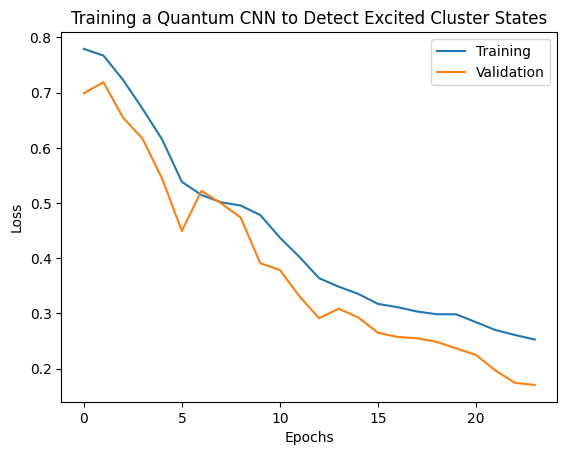
plt.plot(history.history['loss'][1:], label='Training')
plt.plot(history.history['val_loss'][1:], label='Validation')
plt.title('Training a Quantum CNN to Detect Excited Cluster States')
plt.xlabel('Epochs')
plt.ylabel('Loss')
plt.legend()
plt.show()

png

2. হাইব্রিড মডেল

কোয়ান্টাম কনভোলিউশন ব্যবহার করে আপনাকে আট কিউবিট থেকে এক কিউবিটে যেতে হবে না—আপনি কোয়ান্টাম কনভোলিউশনের এক বা দুই রাউন্ড করতে পারতেন এবং ফলাফলগুলিকে একটি ক্লাসিক্যাল নিউরাল নেটওয়ার্কে খাওয়াতে পারতেন। এই বিভাগটি কোয়ান্টাম-ক্লাসিক্যাল হাইব্রিড মডেলগুলি অন্বেষণ করে।

2.1 একটি একক কোয়ান্টাম ফিল্টার সহ হাইব্রিড মডেল

কোয়ান্টাম কনভোলিউশনের একটি স্তর প্রয়োগ করুন, সমস্ত বিটগুলিতে \(\langle \hat{Z}_n \rangle\) পড়ুন, একটি ঘন-সংযুক্ত নিউরাল নেটওয়ার্ক অনুসরণ করুন।

2.1.1 মডেল সংজ্ঞা

# 1-local operators to read out
readouts = [cirq.Z(bit) for bit in cluster_state_bits[4:]]


def multi_readout_model_circuit(qubits):
    """Make a model circuit with less quantum pool and conv operations."""
    model_circuit = cirq.Circuit()
    symbols = sympy.symbols('qconv0:21')
    model_circuit += quantum_conv_circuit(qubits, symbols[0:15])
    model_circuit += quantum_pool_circuit(qubits[:4], qubits[4:],
                                          symbols[15:21])
    return model_circuit


# Build a model enacting the logic in 2.1 of this notebook.
excitation_input_dual = tf.keras.Input(shape=(), dtype=tf.dtypes.string)

cluster_state_dual = tfq.layers.AddCircuit()(
    excitation_input_dual, prepend=cluster_state_circuit(cluster_state_bits))

quantum_model_dual = tfq.layers.PQC(
    multi_readout_model_circuit(cluster_state_bits),
    readouts)(cluster_state_dual)

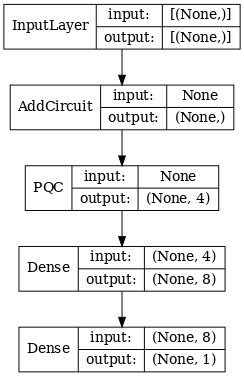
d1_dual = tf.keras.layers.Dense(8)(quantum_model_dual)

d2_dual = tf.keras.layers.Dense(1)(d1_dual)

hybrid_model = tf.keras.Model(inputs=[excitation_input_dual], outputs=[d2_dual])

# Display the model architecture
tf.keras.utils.plot_model(hybrid_model,
                          show_shapes=True,
                          show_layer_names=False,
                          dpi=70)

png

2.1.2 মডেলকে প্রশিক্ষণ দিন

hybrid_model.compile(optimizer=tf.keras.optimizers.Adam(learning_rate=0.02),
                     loss=tf.losses.mse,
                     metrics=[custom_accuracy])

hybrid_history = hybrid_model.fit(x=train_excitations,
                                  y=train_labels,
                                  batch_size=16,
                                  epochs=25,
                                  verbose=1,
                                  validation_data=(test_excitations,
                                                   test_labels))

Epoch 1/25
7/7 [==============================] - 1s 113ms/step - loss: 0.9848 - custom_accuracy: 0.5179 - val_loss: 0.9635 - val_custom_accuracy: 0.5417
Epoch 2/25
7/7 [==============================] - 1s 86ms/step - loss: 0.8095 - custom_accuracy: 0.6339 - val_loss: 0.6800 - val_custom_accuracy: 0.7083
Epoch 3/25
7/7 [==============================] - 1s 85ms/step - loss: 0.4045 - custom_accuracy: 0.9375 - val_loss: 0.3342 - val_custom_accuracy: 0.8750
Epoch 4/25
7/7 [==============================] - 1s 86ms/step - loss: 0.2308 - custom_accuracy: 0.9643 - val_loss: 0.2027 - val_custom_accuracy: 0.9792
Epoch 5/25
7/7 [==============================] - 1s 84ms/step - loss: 0.2232 - custom_accuracy: 0.9554 - val_loss: 0.1761 - val_custom_accuracy: 1.0000
Epoch 6/25
7/7 [==============================] - 1s 84ms/step - loss: 0.1760 - custom_accuracy: 0.9821 - val_loss: 0.2541 - val_custom_accuracy: 0.9167
Epoch 7/25
7/7 [==============================] - 1s 85ms/step - loss: 0.1919 - custom_accuracy: 0.9643 - val_loss: 0.1967 - val_custom_accuracy: 0.9792
Epoch 8/25
7/7 [==============================] - 1s 83ms/step - loss: 0.1892 - custom_accuracy: 0.9554 - val_loss: 0.1870 - val_custom_accuracy: 0.9792
Epoch 9/25
7/7 [==============================] - 1s 84ms/step - loss: 0.1777 - custom_accuracy: 0.9911 - val_loss: 0.2208 - val_custom_accuracy: 0.9583
Epoch 10/25
7/7 [==============================] - 1s 83ms/step - loss: 0.1728 - custom_accuracy: 0.9732 - val_loss: 0.2147 - val_custom_accuracy: 0.9583
Epoch 11/25
7/7 [==============================] - 1s 85ms/step - loss: 0.1704 - custom_accuracy: 0.9732 - val_loss: 0.1810 - val_custom_accuracy: 0.9792
Epoch 12/25
7/7 [==============================] - 1s 85ms/step - loss: 0.1739 - custom_accuracy: 0.9732 - val_loss: 0.2038 - val_custom_accuracy: 0.9792
Epoch 13/25
7/7 [==============================] - 1s 81ms/step - loss: 0.1705 - custom_accuracy: 0.9732 - val_loss: 0.1855 - val_custom_accuracy: 0.9792
Epoch 14/25
7/7 [==============================] - 1s 84ms/step - loss: 0.1788 - custom_accuracy: 0.9643 - val_loss: 0.2152 - val_custom_accuracy: 0.9583
Epoch 15/25
7/7 [==============================] - 1s 84ms/step - loss: 0.1760 - custom_accuracy: 0.9732 - val_loss: 0.1994 - val_custom_accuracy: 1.0000
Epoch 16/25
7/7 [==============================] - 1s 83ms/step - loss: 0.1737 - custom_accuracy: 0.9732 - val_loss: 0.2035 - val_custom_accuracy: 0.9792
Epoch 17/25
7/7 [==============================] - 1s 82ms/step - loss: 0.1749 - custom_accuracy: 0.9911 - val_loss: 0.1983 - val_custom_accuracy: 0.9583
Epoch 18/25
7/7 [==============================] - 1s 83ms/step - loss: 0.1875 - custom_accuracy: 0.9732 - val_loss: 0.1916 - val_custom_accuracy: 0.9583
Epoch 19/25
7/7 [==============================] - 1s 82ms/step - loss: 0.1605 - custom_accuracy: 0.9732 - val_loss: 0.1782 - val_custom_accuracy: 0.9792
Epoch 20/25
7/7 [==============================] - 1s 84ms/step - loss: 0.1668 - custom_accuracy: 0.9911 - val_loss: 0.2276 - val_custom_accuracy: 0.9583
Epoch 21/25
7/7 [==============================] - 1s 84ms/step - loss: 0.1700 - custom_accuracy: 0.9911 - val_loss: 0.2080 - val_custom_accuracy: 0.9583
Epoch 22/25
7/7 [==============================] - 1s 83ms/step - loss: 0.1621 - custom_accuracy: 0.9732 - val_loss: 0.1851 - val_custom_accuracy: 0.9375
Epoch 23/25
7/7 [==============================] - 1s 84ms/step - loss: 0.1695 - custom_accuracy: 0.9911 - val_loss: 0.1882 - val_custom_accuracy: 0.9792
Epoch 24/25
7/7 [==============================] - 1s 82ms/step - loss: 0.1583 - custom_accuracy: 0.9911 - val_loss: 0.2017 - val_custom_accuracy: 0.9583
Epoch 25/25
7/7 [==============================] - 1s 83ms/step - loss: 0.1557 - custom_accuracy: 0.9911 - val_loss: 0.1907 - val_custom_accuracy: 0.9792

plt.plot(history.history['val_custom_accuracy'], label='QCNN')
plt.plot(hybrid_history.history['val_custom_accuracy'], label='Hybrid CNN')
plt.title('Quantum vs Hybrid CNN performance')
plt.xlabel('Epochs')
plt.legend()
plt.ylabel('Validation Accuracy')
plt.show()

png

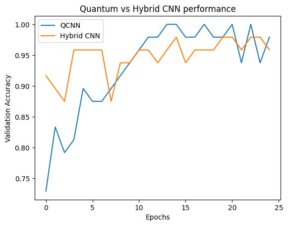
আপনি দেখতে পাচ্ছেন, খুব শালীন শাস্ত্রীয় সহায়তায়, হাইব্রিড মডেলটি সাধারণত বিশুদ্ধভাবে কোয়ান্টাম সংস্করণের চেয়ে দ্রুত একত্রিত হবে।

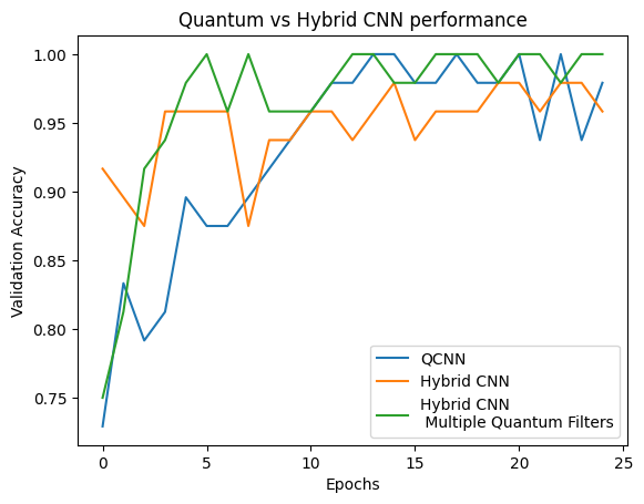
2.2 একাধিক কোয়ান্টাম ফিল্টার সহ হাইব্রিড কনভোলিউশন

এখন আসুন একটি আর্কিটেকচার চেষ্টা করি যা একাধিক কোয়ান্টাম কনভোলিউশন এবং একটি ক্লাসিক্যাল নিউরাল নেটওয়ার্ক ব্যবহার করে তাদের একত্রিত করতে।

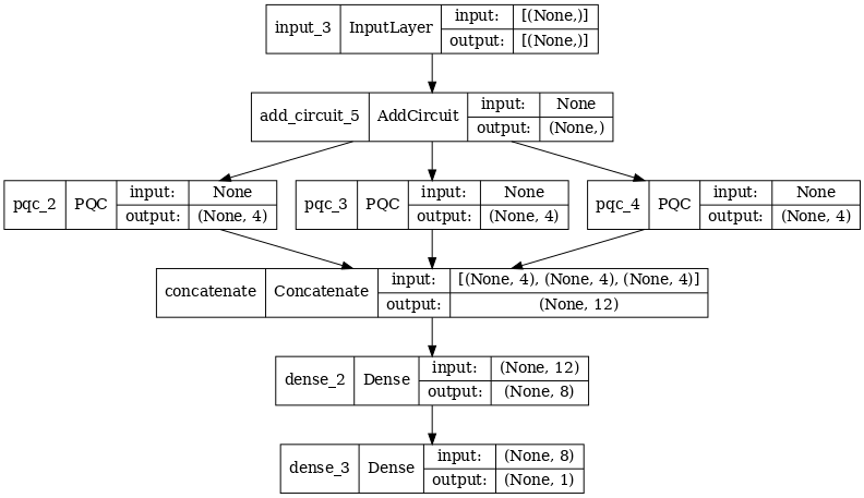
2.2.1 মডেল সংজ্ঞা

excitation_input_multi = tf.keras.Input(shape=(), dtype=tf.dtypes.string)

cluster_state_multi = tfq.layers.AddCircuit()(
    excitation_input_multi, prepend=cluster_state_circuit(cluster_state_bits))

# apply 3 different filters and measure expectation values

quantum_model_multi1 = tfq.layers.PQC(
    multi_readout_model_circuit(cluster_state_bits),
    readouts)(cluster_state_multi)

quantum_model_multi2 = tfq.layers.PQC(
    multi_readout_model_circuit(cluster_state_bits),
    readouts)(cluster_state_multi)

quantum_model_multi3 = tfq.layers.PQC(
    multi_readout_model_circuit(cluster_state_bits),
    readouts)(cluster_state_multi)

# concatenate outputs and feed into a small classical NN
concat_out = tf.keras.layers.concatenate(
    [quantum_model_multi1, quantum_model_multi2, quantum_model_multi3])

dense_1 = tf.keras.layers.Dense(8)(concat_out)

dense_2 = tf.keras.layers.Dense(1)(dense_1)

multi_qconv_model = tf.keras.Model(inputs=[excitation_input_multi],
                                   outputs=[dense_2])

# Display the model architecture
tf.keras.utils.plot_model(multi_qconv_model,
                          show_shapes=True,
                          show_layer_names=True,
                          dpi=70)

png

2.2.2 মডেলকে প্রশিক্ষণ দিন

multi_qconv_model.compile(
    optimizer=tf.keras.optimizers.Adam(learning_rate=0.02),
    loss=tf.losses.mse,
    metrics=[custom_accuracy])

multi_qconv_history = multi_qconv_model.fit(x=train_excitations,
                                            y=train_labels,
                                            batch_size=16,
                                            epochs=25,
                                            verbose=1,
                                            validation_data=(test_excitations,
                                                             test_labels))

Epoch 1/25
7/7 [==============================] - 2s 143ms/step - loss: 0.9425 - custom_accuracy: 0.6429 - val_loss: 0.8120 - val_custom_accuracy: 0.7083
Epoch 2/25
7/7 [==============================] - 1s 109ms/step - loss: 0.5778 - custom_accuracy: 0.7946 - val_loss: 0.5920 - val_custom_accuracy: 0.7500
Epoch 3/25
7/7 [==============================] - 1s 103ms/step - loss: 0.4954 - custom_accuracy: 0.9018 - val_loss: 0.4568 - val_custom_accuracy: 0.7708
Epoch 4/25
7/7 [==============================] - 1s 95ms/step - loss: 0.2855 - custom_accuracy: 0.9196 - val_loss: 0.2792 - val_custom_accuracy: 0.9375
Epoch 5/25
7/7 [==============================] - 1s 93ms/step - loss: 0.1902 - custom_accuracy: 0.9821 - val_loss: 0.2212 - val_custom_accuracy: 0.9375
Epoch 6/25
7/7 [==============================] - 1s 94ms/step - loss: 0.1685 - custom_accuracy: 0.9821 - val_loss: 0.2341 - val_custom_accuracy: 0.9583
Epoch 7/25
7/7 [==============================] - 1s 104ms/step - loss: 0.1671 - custom_accuracy: 0.9911 - val_loss: 0.2062 - val_custom_accuracy: 0.9792
Epoch 8/25
7/7 [==============================] - 1s 97ms/step - loss: 0.1511 - custom_accuracy: 0.9821 - val_loss: 0.2096 - val_custom_accuracy: 0.9792
Epoch 9/25
7/7 [==============================] - 1s 96ms/step - loss: 0.1432 - custom_accuracy: 0.9911 - val_loss: 0.2330 - val_custom_accuracy: 0.9375
Epoch 10/25
7/7 [==============================] - 1s 92ms/step - loss: 0.1668 - custom_accuracy: 0.9821 - val_loss: 0.2344 - val_custom_accuracy: 0.9583
Epoch 11/25
7/7 [==============================] - 1s 106ms/step - loss: 0.1893 - custom_accuracy: 0.9732 - val_loss: 0.2148 - val_custom_accuracy: 0.9583
Epoch 12/25
7/7 [==============================] - 1s 104ms/step - loss: 0.1857 - custom_accuracy: 0.9732 - val_loss: 0.2739 - val_custom_accuracy: 0.9583
Epoch 13/25
7/7 [==============================] - 1s 106ms/step - loss: 0.1748 - custom_accuracy: 0.9732 - val_loss: 0.2366 - val_custom_accuracy: 0.9583
Epoch 14/25
7/7 [==============================] - 1s 103ms/step - loss: 0.1515 - custom_accuracy: 0.9821 - val_loss: 0.2012 - val_custom_accuracy: 0.9583
Epoch 15/25
7/7 [==============================] - 1s 100ms/step - loss: 0.1552 - custom_accuracy: 0.9911 - val_loss: 0.2404 - val_custom_accuracy: 0.9375
Epoch 16/25
7/7 [==============================] - 1s 97ms/step - loss: 0.1572 - custom_accuracy: 0.9911 - val_loss: 0.2779 - val_custom_accuracy: 0.9375
Epoch 17/25
7/7 [==============================] - 1s 100ms/step - loss: 0.1546 - custom_accuracy: 0.9821 - val_loss: 0.2104 - val_custom_accuracy: 0.9583
Epoch 18/25
7/7 [==============================] - 1s 102ms/step - loss: 0.1418 - custom_accuracy: 0.9911 - val_loss: 0.2647 - val_custom_accuracy: 0.9583
Epoch 19/25
7/7 [==============================] - 1s 98ms/step - loss: 0.1590 - custom_accuracy: 0.9732 - val_loss: 0.2154 - val_custom_accuracy: 0.9583
Epoch 20/25
7/7 [==============================] - 1s 104ms/step - loss: 0.1363 - custom_accuracy: 1.0000 - val_loss: 0.2470 - val_custom_accuracy: 0.9375
Epoch 21/25
7/7 [==============================] - 1s 100ms/step - loss: 0.1442 - custom_accuracy: 0.9821 - val_loss: 0.2383 - val_custom_accuracy: 0.9375
Epoch 22/25
7/7 [==============================] - 1s 99ms/step - loss: 0.1415 - custom_accuracy: 0.9911 - val_loss: 0.2324 - val_custom_accuracy: 0.9583
Epoch 23/25
7/7 [==============================] - 1s 97ms/step - loss: 0.1424 - custom_accuracy: 0.9821 - val_loss: 0.2188 - val_custom_accuracy: 0.9583
Epoch 24/25
7/7 [==============================] - 1s 100ms/step - loss: 0.1417 - custom_accuracy: 0.9821 - val_loss: 0.2340 - val_custom_accuracy: 0.9375
Epoch 25/25
7/7 [==============================] - 1s 103ms/step - loss: 0.1471 - custom_accuracy: 0.9732 - val_loss: 0.2252 - val_custom_accuracy: 0.9583

plt.plot(history.history['val_custom_accuracy'][:25], label='QCNN')
plt.plot(hybrid_history.history['val_custom_accuracy'][:25], label='Hybrid CNN')
plt.plot(multi_qconv_history.history['val_custom_accuracy'][:25],
         label='Hybrid CNN \n Multiple Quantum Filters')
plt.title('Quantum vs Hybrid CNN performance')
plt.xlabel('Epochs')
plt.legend()
plt.ylabel('Validation Accuracy')
plt.show()

png