| | |  Kaynağı GitHub'da görüntüleyin Kaynağı GitHub'da görüntüleyin | |
Bu öğretici, aynı zamanda çevirisel olarak değişmez olan klasik bir evrişimsel sinir ağına önerilen bir kuantum analogu olan basitleştirilmiş bir Kuantum Evrişimli Sinir Ağı (QCNN) uygular.
Bu örnek, bir kuantum sensörü veya bir cihazdan karmaşık bir simülasyon gibi bir kuantum veri kaynağının belirli özelliklerinin nasıl tespit edileceğini gösterir. Kuantum veri kaynağı, bir uyarıya sahip olabilen veya olmayabilen bir küme durumudur - QCNN'nin algılamayı öğreneceği şey (Kağıtta kullanılan veri kümesi SPT faz sınıflandırmasıydı).
Kurmak
pip install tensorflow==2.7.0
TensorFlow Quantum'u yükleyin:
pip install tensorflow-quantum
# Update package resources to account for version changes.
import importlib, pkg_resources
importlib.reload(pkg_resources)
<module 'pkg_resources' from '/tmpfs/src/tf_docs_env/lib/python3.7/site-packages/pkg_resources/__init__.py'>
Şimdi TensorFlow ve modül bağımlılıklarını içe aktarın:
import tensorflow as tf
import tensorflow_quantum as tfq

import cirq
import sympy
import numpy as np

# visualization tools
%matplotlib inline
import matplotlib.pyplot as plt
from cirq.contrib.svg import SVGCircuit
2022-02-04 12:43:45.380301: E tensorflow/stream_executor/cuda/cuda_driver.cc:271] failed call to cuInit: CUDA_ERROR_NO_DEVICE: no CUDA-capable device is detected
1. Bir QCNN oluşturun
1.1 Devreleri TensorFlow grafiğinde birleştirme
TensorFlow Quantum (TFQ), grafik içi devre yapımı için tasarlanmış katman sınıfları sağlar. Bir örnek, tf.keras.Layer öğesinden miras alan tfq.layers.AddCircuit tf.keras.Layer . Bu katman, aşağıdaki şekilde gösterildiği gibi, devrelerin giriş partisinin başına veya sonuna eklenebilir.
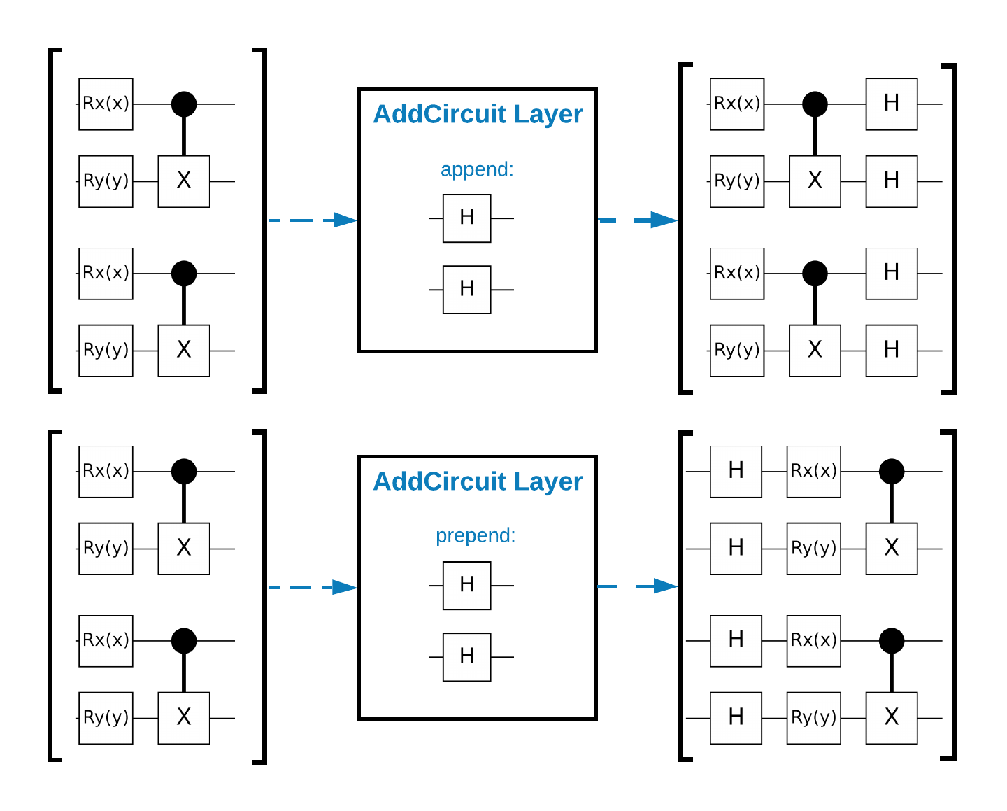
Aşağıdaki kod parçası bu katmanı kullanır:
qubit = cirq.GridQubit(0, 0)

# Define some circuits.
circuit1 = cirq.Circuit(cirq.X(qubit))
circuit2 = cirq.Circuit(cirq.H(qubit))

# Convert to a tensor.
input_circuit_tensor = tfq.convert_to_tensor([circuit1, circuit2])

# Define a circuit that we want to append
y_circuit = cirq.Circuit(cirq.Y(qubit))

# Instantiate our layer
y_appender = tfq.layers.AddCircuit()

# Run our circuit tensor through the layer and save the output.
output_circuit_tensor = y_appender(input_circuit_tensor, append=y_circuit)
Giriş tensörünü inceleyin:
print(tfq.from_tensor(input_circuit_tensor))
[cirq.Circuit([
     cirq.Moment(
         cirq.X(cirq.GridQubit(0, 0)),
     ),
 ])
 cirq.Circuit([
     cirq.Moment(
         cirq.H(cirq.GridQubit(0, 0)),
     ),
 ])                                   ]
Ve çıkış tensörünü inceleyin:
print(tfq.from_tensor(output_circuit_tensor))
[cirq.Circuit([
     cirq.Moment(
         cirq.X(cirq.GridQubit(0, 0)),
     ),
     cirq.Moment(
         cirq.Y(cirq.GridQubit(0, 0)),
     ),
 ])
 cirq.Circuit([
     cirq.Moment(
         cirq.H(cirq.GridQubit(0, 0)),
     ),
     cirq.Moment(
         cirq.Y(cirq.GridQubit(0, 0)),
     ),
 ])                                   ]
Aşağıdaki örnekleri tfq.layers.AddCircuit kullanmadan çalıştırmak mümkün olsa da, karmaşık işlevlerin TensorFlow hesaplama grafiklerine nasıl yerleştirilebileceğini anlamak için iyi bir fırsat.
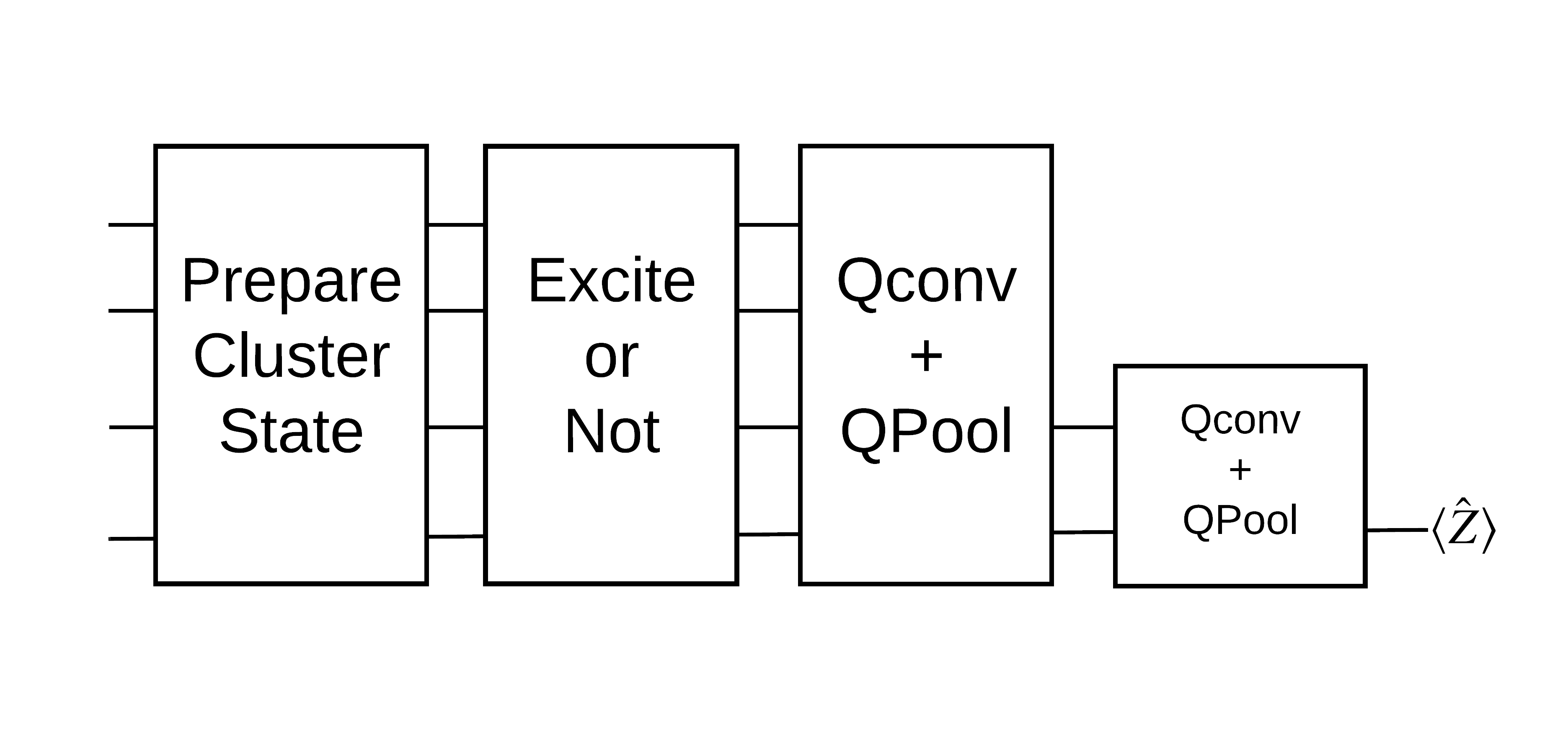
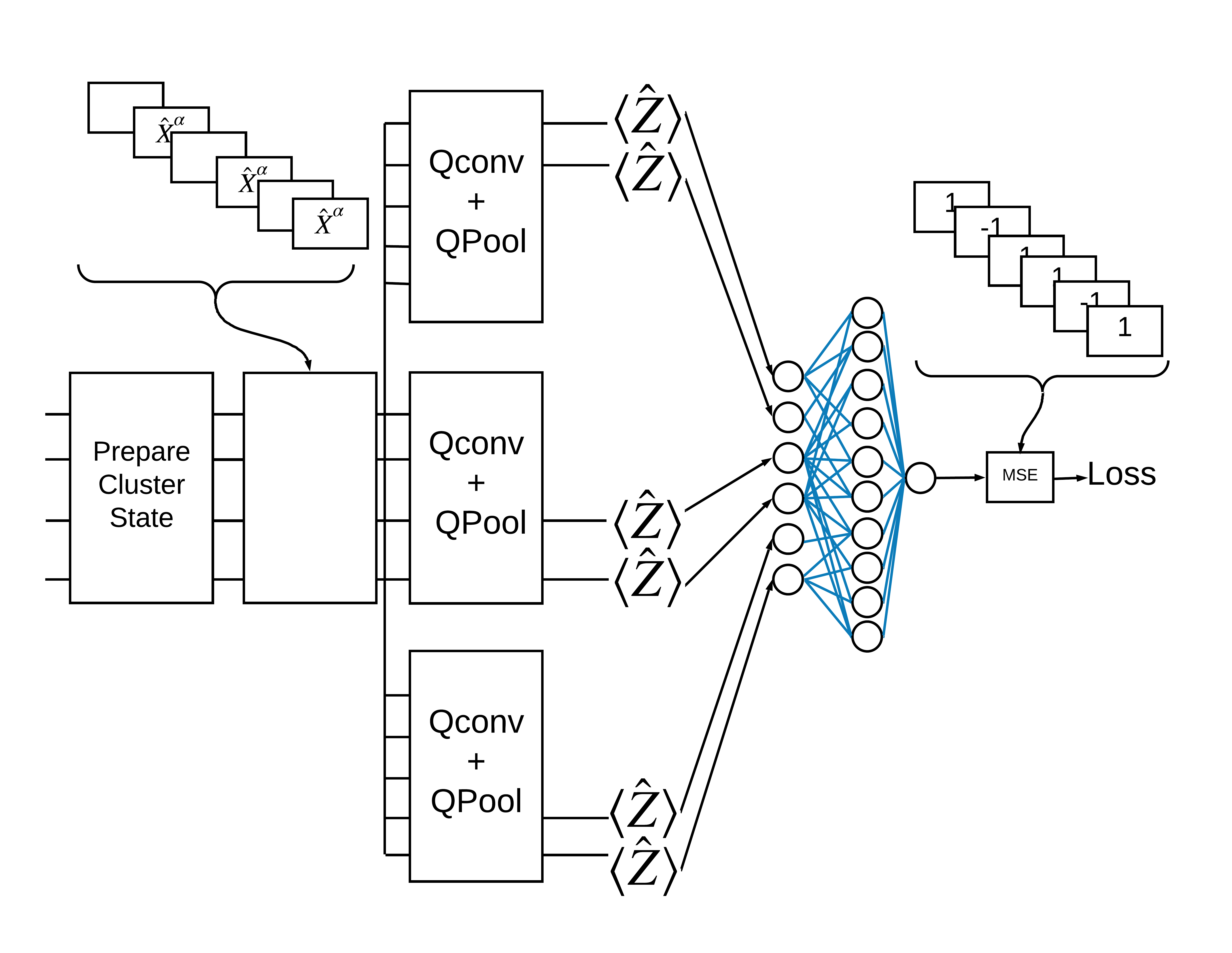
1.2 Soruna genel bakış
Bir küme durumu hazırlayacak ve "heyecanlı" olup olmadığını saptamak için bir kuantum sınıflandırıcı eğiteceksiniz. Küme durumu oldukça karışıktır ancak klasik bir bilgisayar için mutlaka zor değildir. Anlaşılır olması açısından bu, makalede kullanılandan daha basit bir veri kümesidir.
Bu sınıflandırma görevi için derin bir MERA benzeri QCNN mimarisi uygulayacaksınız, çünkü:
- QCNN gibi, bir halkadaki küme durumu da öteleme açısından değişmezdir.
- Küme durumu oldukça karışık.
Bu mimari, tek bir kübiti okuyarak sınıflandırmayı elde ederek dolaşıklığı azaltmada etkili olmalıdır.
"Uyarılmış" bir küme durumu, herhangi bir kübitine uygulanan bir cirq.rx kapısına sahip bir küme durumu olarak tanımlanır. Qconv ve QPool bu öğreticide daha sonra tartışılacaktır.
1.3 TensorFlow için yapı taşları
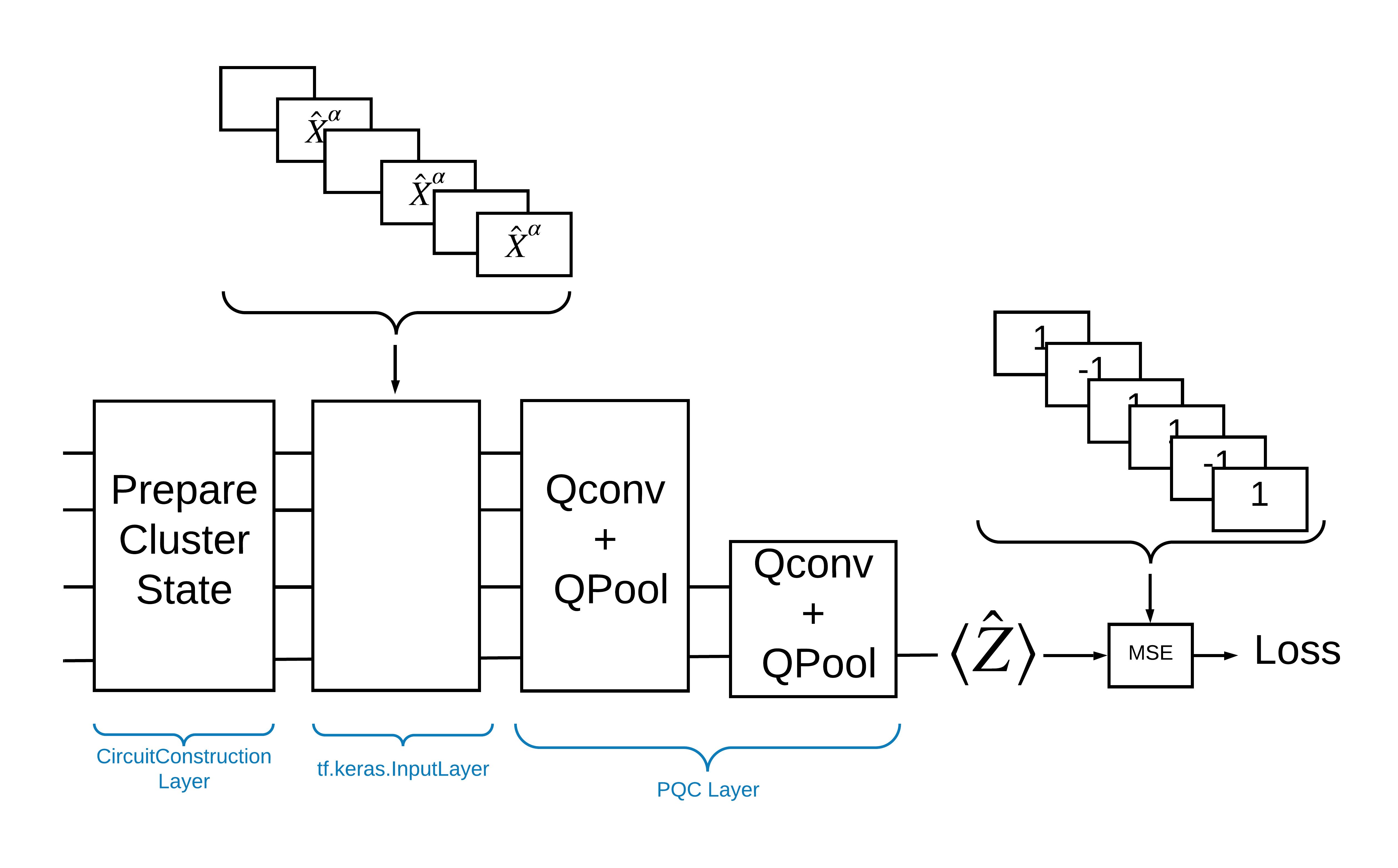
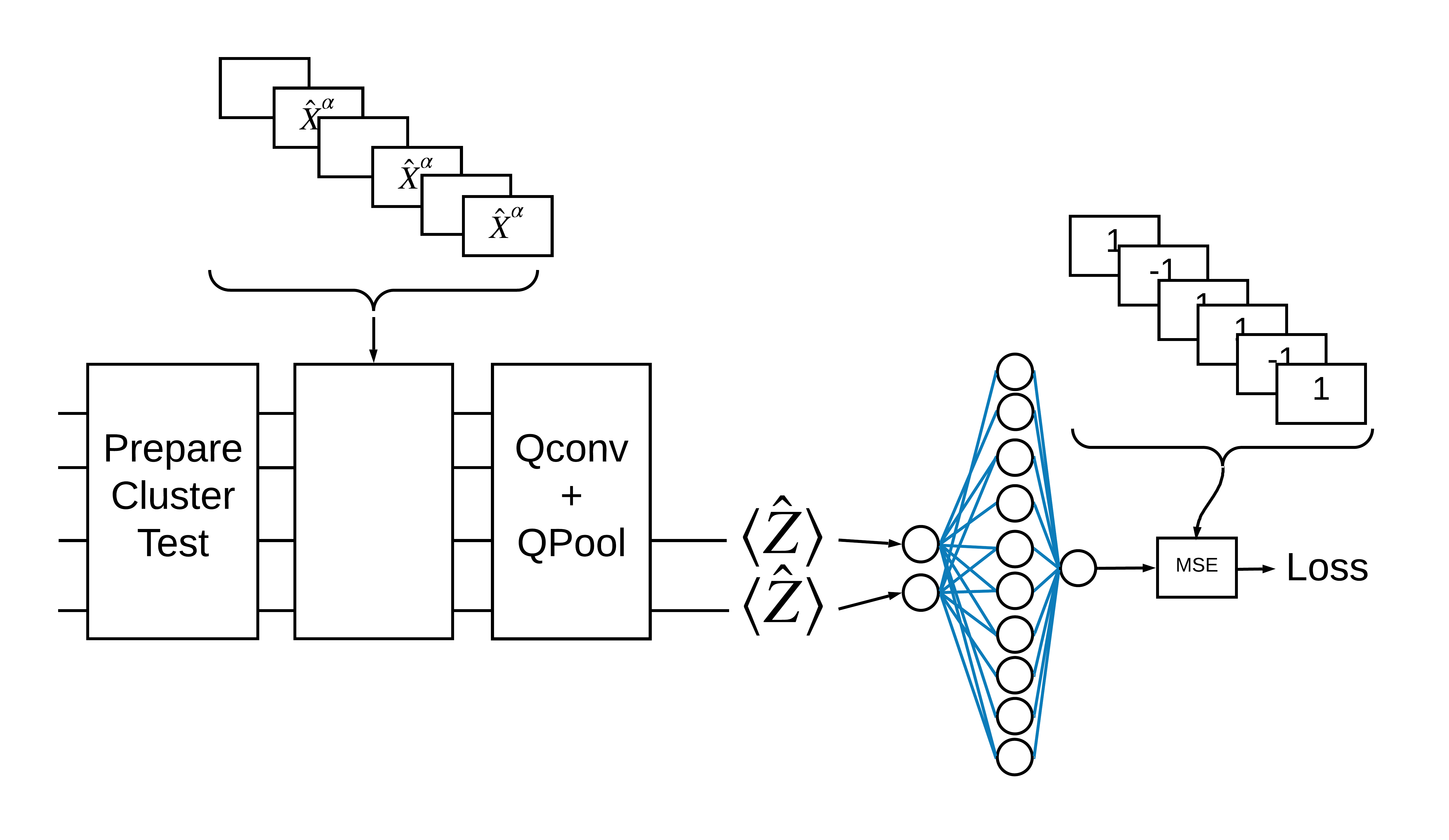
Bu sorunu TensorFlow Quantum ile çözmenin bir yolu aşağıdakileri uygulamaktır:
- Modelin girdisi bir devre tensörüdür - ya boş bir devre ya da belirli bir kübit üzerindeki bir uyarımı gösteren bir X kapısı.
- Modelin kuantum bileşenlerinin geri kalanı
tfq.layers.AddCircuitkatmanlarıyla oluşturulmuştur. - Çıkarım için bir
tfq.layers.PQCkatmanı kullanılır. Bu, \(\langle \hat{Z} \rangle\) okur ve uyarılmış bir durum için 1 veya uyarılmamış bir durum için -1 etiketiyle karşılaştırır.
1.4 Veri
Modelinizi oluşturmadan önce verilerinizi oluşturabilirsiniz. Bu durumda küme durumuna yönelik uyarılar olacaktır (Orijinal makale daha karmaşık bir veri kümesi kullanır). cirq.rx kapıları ile temsil edilir. Yeterince büyük bir dönüş bir uyarı olarak kabul edilir ve 1 olarak etiketlenir ve yeterince büyük olmayan bir dönüş -1 olarak etiketlenir ve bir uyarı olarak kabul edilmez.
def generate_data(qubits):
    """Generate training and testing data."""
    n_rounds = 20  # Produces n_rounds * n_qubits datapoints.
    excitations = []
    labels = []
    for n in range(n_rounds):
        for bit in qubits:
            rng = np.random.uniform(-np.pi, np.pi)
            excitations.append(cirq.Circuit(cirq.rx(rng)(bit)))
            labels.append(1 if (-np.pi / 2) <= rng <= (np.pi / 2) else -1)

    split_ind = int(len(excitations) * 0.7)
    train_excitations = excitations[:split_ind]
    test_excitations = excitations[split_ind:]

    train_labels = labels[:split_ind]
    test_labels = labels[split_ind:]

    return tfq.convert_to_tensor(train_excitations), np.array(train_labels), \
        tfq.convert_to_tensor(test_excitations), np.array(test_labels)
Tıpkı normal makine öğreniminde olduğu gibi, modeli kıyaslamak için kullanmak üzere bir eğitim ve test seti oluşturduğunuzu görebilirsiniz. Aşağıdakilerle bazı veri noktalarına hızlıca bakabilirsiniz:
sample_points, sample_labels, _, __ = generate_data(cirq.GridQubit.rect(1, 4))
print('Input:', tfq.from_tensor(sample_points)[0], 'Output:', sample_labels[0])
print('Input:', tfq.from_tensor(sample_points)[1], 'Output:', sample_labels[1])
Input: (0, 0): ───X^0.449─── Output: 1
Input: (0, 1): ───X^-0.74─── Output: -1
1.5 Katmanları tanımlayın
Şimdi yukarıdaki şekilde gösterilen katmanları TensorFlow'da tanımlayın.
1.5.1 Küme durumu
İlk adım, kuantum devrelerini programlamak için Google tarafından sağlanan bir çerçeve olan Cirq'i kullanarak küme durumunu tanımlamaktır. Bu, modelin statik bir parçası olduğundan, onu tfq.layers.AddCircuit işlevini kullanarak gömün.
def cluster_state_circuit(bits):
    """Return a cluster state on the qubits in `bits`."""
    circuit = cirq.Circuit()
    circuit.append(cirq.H.on_each(bits))
    for this_bit, next_bit in zip(bits, bits[1:] + [bits[0]]):
        circuit.append(cirq.CZ(this_bit, next_bit))
    return circuit
cirq.GridQubit s dikdörtgeni için bir küme durumu devresi görüntüleyin:
SVGCircuit(cluster_state_circuit(cirq.GridQubit.rect(1, 4)))
findfont: Font family ['Arial'] not found. Falling back to DejaVu Sans.

1.5.2 QCNN katmanları
Cong ve Lukin QCNN kağıdını kullanarak modeli oluşturan katmanları tanımlayın. Birkaç önkoşul vardır:
- Tucci makalesinden bir ve iki kübitlik parametreli üniter matrisler.
- Genel bir parametreli iki kübit havuzlama işlemi.
def one_qubit_unitary(bit, symbols):
    """Make a Cirq circuit enacting a rotation of the bloch sphere about the X,
    Y and Z axis, that depends on the values in `symbols`.
    """
    return cirq.Circuit(
        cirq.X(bit)**symbols[0],
        cirq.Y(bit)**symbols[1],
        cirq.Z(bit)**symbols[2])


def two_qubit_unitary(bits, symbols):
    """Make a Cirq circuit that creates an arbitrary two qubit unitary."""
    circuit = cirq.Circuit()
    circuit += one_qubit_unitary(bits[0], symbols[0:3])
    circuit += one_qubit_unitary(bits[1], symbols[3:6])
    circuit += [cirq.ZZ(*bits)**symbols[6]]
    circuit += [cirq.YY(*bits)**symbols[7]]
    circuit += [cirq.XX(*bits)**symbols[8]]
    circuit += one_qubit_unitary(bits[0], symbols[9:12])
    circuit += one_qubit_unitary(bits[1], symbols[12:])
    return circuit


def two_qubit_pool(source_qubit, sink_qubit, symbols):
    """Make a Cirq circuit to do a parameterized 'pooling' operation, which
    attempts to reduce entanglement down from two qubits to just one."""
    pool_circuit = cirq.Circuit()
    sink_basis_selector = one_qubit_unitary(sink_qubit, symbols[0:3])
    source_basis_selector = one_qubit_unitary(source_qubit, symbols[3:6])
    pool_circuit.append(sink_basis_selector)
    pool_circuit.append(source_basis_selector)
    pool_circuit.append(cirq.CNOT(control=source_qubit, target=sink_qubit))
    pool_circuit.append(sink_basis_selector**-1)
    return pool_circuit
Ne yarattığınızı görmek için tek kübitlik üniter devreyi yazdırın:
SVGCircuit(one_qubit_unitary(cirq.GridQubit(0, 0), sympy.symbols('x0:3')))

Ve iki kübitlik üniter devre:
SVGCircuit(two_qubit_unitary(cirq.GridQubit.rect(1, 2), sympy.symbols('x0:15')))

Ve iki kübit havuzlama devresi:
SVGCircuit(two_qubit_pool(*cirq.GridQubit.rect(1, 2), sympy.symbols('x0:6')))

1.5.2.1 Kuantum evrişim
Cong ve Lukin makalesinde olduğu gibi, 1B kuantum evrişimini, iki kübitlik parametreli bir ünitenin, bir adımlık her bitişik kübit çiftine uygulanması olarak tanımlayın.
def quantum_conv_circuit(bits, symbols):
    """Quantum Convolution Layer following the above diagram.
    Return a Cirq circuit with the cascade of `two_qubit_unitary` applied
    to all pairs of qubits in `bits` as in the diagram above.
    """
    circuit = cirq.Circuit()
    for first, second in zip(bits[0::2], bits[1::2]):
        circuit += two_qubit_unitary([first, second], symbols)
    for first, second in zip(bits[1::2], bits[2::2] + [bits[0]]):
        circuit += two_qubit_unitary([first, second], symbols)
    return circuit
(çok yatay) devreyi görüntüleyin:
SVGCircuit(
    quantum_conv_circuit(cirq.GridQubit.rect(1, 8), sympy.symbols('x0:15')))

1.5.2.2 Kuantum havuzu
Bir kuantum havuzlama katmanı, yukarıda tanımlanan iki kübitlik havuzu kullanarak l10n \(N\) yer tutucu2 kübitlerden \(\frac{N}{2}\) tutucu3 kübitlere havuzlar.
def quantum_pool_circuit(source_bits, sink_bits, symbols):
    """A layer that specifies a quantum pooling operation.
    A Quantum pool tries to learn to pool the relevant information from two
    qubits onto 1.
    """
    circuit = cirq.Circuit()
    for source, sink in zip(source_bits, sink_bits):
        circuit += two_qubit_pool(source, sink, symbols)
    return circuit
Bir havuzlama bileşen devresini inceleyin:
test_bits = cirq.GridQubit.rect(1, 8)

SVGCircuit(
    quantum_pool_circuit(test_bits[:4], test_bits[4:], sympy.symbols('x0:6')))

1.6 Model tanımı
Şimdi tamamen kuantum bir CNN oluşturmak için tanımlanmış katmanları kullanın. Sekiz kübitle başlayın, bire indirgeyin, ardından \(\langle \hat{Z} \rangle\)ölçün.
def create_model_circuit(qubits):
"""Create sequence of alternating convolution and pooling operators
which gradually shrink over time."""
model_circuit = cirq.Circuit()
symbols = sympy.symbols('qconv0:63')
# Cirq uses sympy.Symbols to map learnable variables. TensorFlow Quantum
# scans incoming circuits and replaces these with TensorFlow variables.
model_circuit += quantum_conv_circuit(qubits, symbols[0:15])
model_circuit += quantum_pool_circuit(qubits[:4], qubits[4:],
symbols[15:21])
model_circuit += quantum_conv_circuit(qubits[4:], symbols[21:36])
model_circuit += quantum_pool_circuit(qubits[4:6], qubits[6:],
symbols[36:42])
model_circuit += quantum_conv_circuit(qubits[6:], symbols[42:57])
model_circuit += quantum_pool_circuit([qubits[6]], [qubits[7]],
symbols[57:63])
return model_circuit
# Create our qubits and readout operators in Cirq.
cluster_state_bits = cirq.GridQubit.rect(1, 8)
readout_operators = cirq.Z(cluster_state_bits[-1])
# Build a sequential model enacting the logic in 1.3 of this notebook.
# Here you are making the static cluster state prep as a part of the AddCircuit and the
# "quantum datapoints" are coming in the form of excitation
excitation_input = tf.keras.Input(shape=(), dtype=tf.dtypes.string)
cluster_state = tfq.layers.AddCircuit()(
excitation_input, prepend=cluster_state_circuit(cluster_state_bits))
quantum_model = tfq.layers.PQC(create_model_circuit(cluster_state_bits),
readout_operators)(cluster_state)
qcnn_model = tf.keras.Model(inputs=[excitation_input], outputs=[quantum_model])
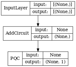
# Show the keras plot of the model
tf.keras.utils.plot_model(qcnn_model,
show_shapes=True,
show_layer_names=False,
dpi=70)
1.7 Modeli eğitin
Bu örneği basitleştirmek için modeli tam parti üzerinde eğitin.
# Generate some training data.
train_excitations, train_labels, test_excitations, test_labels = generate_data(
    cluster_state_bits)


# Custom accuracy metric.
@tf.function
def custom_accuracy(y_true, y_pred):
    y_true = tf.squeeze(y_true)
    y_pred = tf.map_fn(lambda x: 1.0 if x >= 0 else -1.0, y_pred)
    return tf.keras.backend.mean(tf.keras.backend.equal(y_true, y_pred))


qcnn_model.compile(optimizer=tf.keras.optimizers.Adam(learning_rate=0.02),
                   loss=tf.losses.mse,
                   metrics=[custom_accuracy])

history = qcnn_model.fit(x=train_excitations,
                         y=train_labels,
                         batch_size=16,
                         epochs=25,
                         verbose=1,
                         validation_data=(test_excitations, test_labels))
Epoch 1/25
7/7 [==============================] - 2s 176ms/step - loss: 0.8961 - custom_accuracy: 0.7143 - val_loss: 0.8012 - val_custom_accuracy: 0.7500
Epoch 2/25
7/7 [==============================] - 1s 140ms/step - loss: 0.7736 - custom_accuracy: 0.7946 - val_loss: 0.7355 - val_custom_accuracy: 0.8542
Epoch 3/25
7/7 [==============================] - 1s 138ms/step - loss: 0.7319 - custom_accuracy: 0.8393 - val_loss: 0.7045 - val_custom_accuracy: 0.8125
Epoch 4/25
7/7 [==============================] - 1s 137ms/step - loss: 0.6976 - custom_accuracy: 0.8482 - val_loss: 0.6829 - val_custom_accuracy: 0.8333
Epoch 5/25
7/7 [==============================] - 1s 143ms/step - loss: 0.6696 - custom_accuracy: 0.8750 - val_loss: 0.6749 - val_custom_accuracy: 0.7917
Epoch 6/25
7/7 [==============================] - 1s 137ms/step - loss: 0.6631 - custom_accuracy: 0.8750 - val_loss: 0.6718 - val_custom_accuracy: 0.7917
Epoch 7/25
7/7 [==============================] - 1s 135ms/step - loss: 0.6536 - custom_accuracy: 0.8929 - val_loss: 0.6638 - val_custom_accuracy: 0.8750
Epoch 8/25
7/7 [==============================] - 1s 141ms/step - loss: 0.6376 - custom_accuracy: 0.8750 - val_loss: 0.6311 - val_custom_accuracy: 0.8542
Epoch 9/25
7/7 [==============================] - 1s 137ms/step - loss: 0.6208 - custom_accuracy: 0.8750 - val_loss: 0.5995 - val_custom_accuracy: 0.8542
Epoch 10/25
7/7 [==============================] - 1s 134ms/step - loss: 0.5887 - custom_accuracy: 0.8661 - val_loss: 0.5655 - val_custom_accuracy: 0.8333
Epoch 11/25
7/7 [==============================] - 1s 144ms/step - loss: 0.5796 - custom_accuracy: 0.8482 - val_loss: 0.5681 - val_custom_accuracy: 0.8333
Epoch 12/25
7/7 [==============================] - 1s 143ms/step - loss: 0.5630 - custom_accuracy: 0.7946 - val_loss: 0.5179 - val_custom_accuracy: 0.8333
Epoch 13/25
7/7 [==============================] - 1s 137ms/step - loss: 0.5405 - custom_accuracy: 0.8304 - val_loss: 0.5003 - val_custom_accuracy: 0.8333
Epoch 14/25
7/7 [==============================] - 1s 138ms/step - loss: 0.5259 - custom_accuracy: 0.8036 - val_loss: 0.4787 - val_custom_accuracy: 0.8333
Epoch 15/25
7/7 [==============================] - 1s 137ms/step - loss: 0.5077 - custom_accuracy: 0.8482 - val_loss: 0.4741 - val_custom_accuracy: 0.8125
Epoch 16/25
7/7 [==============================] - 1s 136ms/step - loss: 0.5082 - custom_accuracy: 0.8214 - val_loss: 0.4739 - val_custom_accuracy: 0.8125
Epoch 17/25
7/7 [==============================] - 1s 137ms/step - loss: 0.5138 - custom_accuracy: 0.8214 - val_loss: 0.4859 - val_custom_accuracy: 0.8750
Epoch 18/25
7/7 [==============================] - 1s 133ms/step - loss: 0.5073 - custom_accuracy: 0.8304 - val_loss: 0.4879 - val_custom_accuracy: 0.8333
Epoch 19/25
7/7 [==============================] - 1s 138ms/step - loss: 0.5084 - custom_accuracy: 0.8304 - val_loss: 0.4745 - val_custom_accuracy: 0.8542
Epoch 20/25
7/7 [==============================] - 1s 139ms/step - loss: 0.5057 - custom_accuracy: 0.8571 - val_loss: 0.4702 - val_custom_accuracy: 0.8333
Epoch 21/25
7/7 [==============================] - 1s 135ms/step - loss: 0.4939 - custom_accuracy: 0.8304 - val_loss: 0.4734 - val_custom_accuracy: 0.8750
Epoch 22/25
7/7 [==============================] - 1s 138ms/step - loss: 0.4942 - custom_accuracy: 0.8750 - val_loss: 0.4725 - val_custom_accuracy: 0.8750
Epoch 23/25
7/7 [==============================] - 1s 140ms/step - loss: 0.4982 - custom_accuracy: 0.9107 - val_loss: 0.4695 - val_custom_accuracy: 0.8958
Epoch 24/25
7/7 [==============================] - 1s 135ms/step - loss: 0.4936 - custom_accuracy: 0.8661 - val_loss: 0.4731 - val_custom_accuracy: 0.8750
Epoch 25/25
7/7 [==============================] - 1s 136ms/step - loss: 0.4866 - custom_accuracy: 0.8571 - val_loss: 0.4631 - val_custom_accuracy: 0.8958
-yer tutucu33 l10n-yer
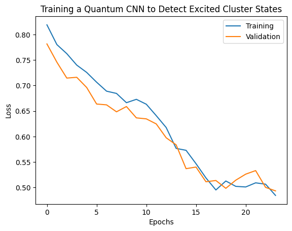
plt.plot(history.history['loss'][1:], label='Training')
plt.plot(history.history['val_loss'][1:], label='Validation')
plt.title('Training a Quantum CNN to Detect Excited Cluster States')
plt.xlabel('Epochs')
plt.ylabel('Loss')
plt.legend()
plt.show()
2. Hibrit modeller
Kuantum evrişimi kullanarak sekiz kübitten bir kübite gitmek zorunda değilsiniz - bir veya iki tur kuantum evrişimi yapabilir ve sonuçları klasik bir sinir ağına besleyebilirdiniz. Bu bölüm kuantum-klasik hibrit modelleri incelemektedir.
2.1 Tek bir kuantum filtreli hibrit model
Tüm bitlerde \(\langle \hat{Z}_n \rangle\) okuyarak bir kuantum evrişim katmanı uygulayın ve ardından yoğun bağlantılı bir sinir ağı uygulayın.
2.1.1 Model tanımı
# 1-local operators to read out
readouts = [cirq.Z(bit) for bit in cluster_state_bits[4:]]
def multi_readout_model_circuit(qubits):
"""Make a model circuit with less quantum pool and conv operations."""
model_circuit = cirq.Circuit()
symbols = sympy.symbols('qconv0:21')
model_circuit += quantum_conv_circuit(qubits, symbols[0:15])
model_circuit += quantum_pool_circuit(qubits[:4], qubits[4:],
symbols[15:21])
return model_circuit
# Build a model enacting the logic in 2.1 of this notebook.
excitation_input_dual = tf.keras.Input(shape=(), dtype=tf.dtypes.string)
cluster_state_dual = tfq.layers.AddCircuit()(
excitation_input_dual, prepend=cluster_state_circuit(cluster_state_bits))
quantum_model_dual = tfq.layers.PQC(
multi_readout_model_circuit(cluster_state_bits),
readouts)(cluster_state_dual)
d1_dual = tf.keras.layers.Dense(8)(quantum_model_dual)
d2_dual = tf.keras.layers.Dense(1)(d1_dual)
hybrid_model = tf.keras.Model(inputs=[excitation_input_dual], outputs=[d2_dual])
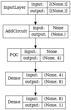
# Display the model architecture
tf.keras.utils.plot_model(hybrid_model,
show_shapes=True,
show_layer_names=False,
dpi=70)
2.1.2 Modeli eğitin
hybrid_model.compile(optimizer=tf.keras.optimizers.Adam(learning_rate=0.02),
                     loss=tf.losses.mse,
                     metrics=[custom_accuracy])

hybrid_history = hybrid_model.fit(x=train_excitations,
                                  y=train_labels,
                                  batch_size=16,
                                  epochs=25,
                                  verbose=1,
                                  validation_data=(test_excitations,
                                                   test_labels))
Epoch 1/25
7/7 [==============================] - 1s 113ms/step - loss: 0.9848 - custom_accuracy: 0.5179 - val_loss: 0.9635 - val_custom_accuracy: 0.5417
Epoch 2/25
7/7 [==============================] - 1s 86ms/step - loss: 0.8095 - custom_accuracy: 0.6339 - val_loss: 0.6800 - val_custom_accuracy: 0.7083
Epoch 3/25
7/7 [==============================] - 1s 85ms/step - loss: 0.4045 - custom_accuracy: 0.9375 - val_loss: 0.3342 - val_custom_accuracy: 0.8750
Epoch 4/25
7/7 [==============================] - 1s 86ms/step - loss: 0.2308 - custom_accuracy: 0.9643 - val_loss: 0.2027 - val_custom_accuracy: 0.9792
Epoch 5/25
7/7 [==============================] - 1s 84ms/step - loss: 0.2232 - custom_accuracy: 0.9554 - val_loss: 0.1761 - val_custom_accuracy: 1.0000
Epoch 6/25
7/7 [==============================] - 1s 84ms/step - loss: 0.1760 - custom_accuracy: 0.9821 - val_loss: 0.2541 - val_custom_accuracy: 0.9167
Epoch 7/25
7/7 [==============================] - 1s 85ms/step - loss: 0.1919 - custom_accuracy: 0.9643 - val_loss: 0.1967 - val_custom_accuracy: 0.9792
Epoch 8/25
7/7 [==============================] - 1s 83ms/step - loss: 0.1892 - custom_accuracy: 0.9554 - val_loss: 0.1870 - val_custom_accuracy: 0.9792
Epoch 9/25
7/7 [==============================] - 1s 84ms/step - loss: 0.1777 - custom_accuracy: 0.9911 - val_loss: 0.2208 - val_custom_accuracy: 0.9583
Epoch 10/25
7/7 [==============================] - 1s 83ms/step - loss: 0.1728 - custom_accuracy: 0.9732 - val_loss: 0.2147 - val_custom_accuracy: 0.9583
Epoch 11/25
7/7 [==============================] - 1s 85ms/step - loss: 0.1704 - custom_accuracy: 0.9732 - val_loss: 0.1810 - val_custom_accuracy: 0.9792
Epoch 12/25
7/7 [==============================] - 1s 85ms/step - loss: 0.1739 - custom_accuracy: 0.9732 - val_loss: 0.2038 - val_custom_accuracy: 0.9792
Epoch 13/25
7/7 [==============================] - 1s 81ms/step - loss: 0.1705 - custom_accuracy: 0.9732 - val_loss: 0.1855 - val_custom_accuracy: 0.9792
Epoch 14/25
7/7 [==============================] - 1s 84ms/step - loss: 0.1788 - custom_accuracy: 0.9643 - val_loss: 0.2152 - val_custom_accuracy: 0.9583
Epoch 15/25
7/7 [==============================] - 1s 84ms/step - loss: 0.1760 - custom_accuracy: 0.9732 - val_loss: 0.1994 - val_custom_accuracy: 1.0000
Epoch 16/25
7/7 [==============================] - 1s 83ms/step - loss: 0.1737 - custom_accuracy: 0.9732 - val_loss: 0.2035 - val_custom_accuracy: 0.9792
Epoch 17/25
7/7 [==============================] - 1s 82ms/step - loss: 0.1749 - custom_accuracy: 0.9911 - val_loss: 0.1983 - val_custom_accuracy: 0.9583
Epoch 18/25
7/7 [==============================] - 1s 83ms/step - loss: 0.1875 - custom_accuracy: 0.9732 - val_loss: 0.1916 - val_custom_accuracy: 0.9583
Epoch 19/25
7/7 [==============================] - 1s 82ms/step - loss: 0.1605 - custom_accuracy: 0.9732 - val_loss: 0.1782 - val_custom_accuracy: 0.9792
Epoch 20/25
7/7 [==============================] - 1s 84ms/step - loss: 0.1668 - custom_accuracy: 0.9911 - val_loss: 0.2276 - val_custom_accuracy: 0.9583
Epoch 21/25
7/7 [==============================] - 1s 84ms/step - loss: 0.1700 - custom_accuracy: 0.9911 - val_loss: 0.2080 - val_custom_accuracy: 0.9583
Epoch 22/25
7/7 [==============================] - 1s 83ms/step - loss: 0.1621 - custom_accuracy: 0.9732 - val_loss: 0.1851 - val_custom_accuracy: 0.9375
Epoch 23/25
7/7 [==============================] - 1s 84ms/step - loss: 0.1695 - custom_accuracy: 0.9911 - val_loss: 0.1882 - val_custom_accuracy: 0.9792
Epoch 24/25
7/7 [==============================] - 1s 82ms/step - loss: 0.1583 - custom_accuracy: 0.9911 - val_loss: 0.2017 - val_custom_accuracy: 0.9583
Epoch 25/25
7/7 [==============================] - 1s 83ms/step - loss: 0.1557 - custom_accuracy: 0.9911 - val_loss: 0.1907 - val_custom_accuracy: 0.9792
-yer tutucu37 l10n-yer
plt.plot(history.history['val_custom_accuracy'], label='QCNN')
plt.plot(hybrid_history.history['val_custom_accuracy'], label='Hybrid CNN')
plt.title('Quantum vs Hybrid CNN performance')
plt.xlabel('Epochs')
plt.legend()
plt.ylabel('Validation Accuracy')
plt.show()
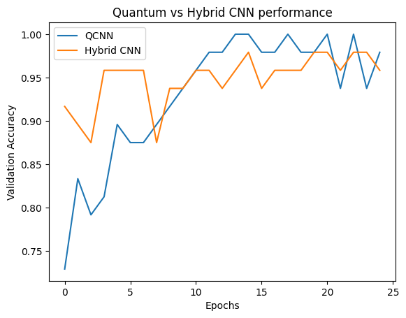
Gördüğünüz gibi, çok mütevazı bir klasik yardımla, hibrit model genellikle tamamen kuantum versiyonundan daha hızlı yakınsayacaktır.
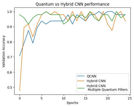
2.2 Çoklu kuantum filtreli hibrit evrişim
Şimdi bunları birleştirmek için çoklu kuantum evrişimlerini ve klasik bir sinir ağını kullanan bir mimari deneyelim.
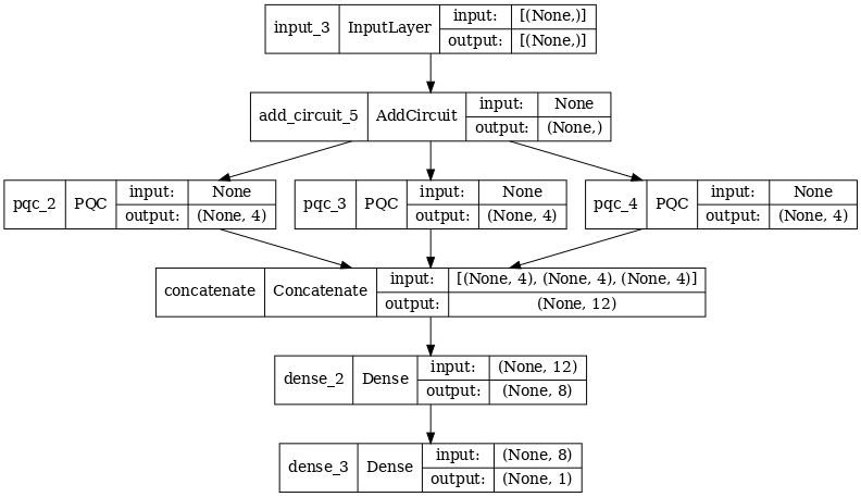
2.2.1 Model tanımı
excitation_input_multi = tf.keras.Input(shape=(), dtype=tf.dtypes.string)

cluster_state_multi = tfq.layers.AddCircuit()(
    excitation_input_multi, prepend=cluster_state_circuit(cluster_state_bits))

# apply 3 different filters and measure expectation values

quantum_model_multi1 = tfq.layers.PQC(
    multi_readout_model_circuit(cluster_state_bits),
    readouts)(cluster_state_multi)

quantum_model_multi2 = tfq.layers.PQC(
    multi_readout_model_circuit(cluster_state_bits),
    readouts)(cluster_state_multi)

quantum_model_multi3 = tfq.layers.PQC(
    multi_readout_model_circuit(cluster_state_bits),
    readouts)(cluster_state_multi)

# concatenate outputs and feed into a small classical NN
concat_out = tf.keras.layers.concatenate(
    [quantum_model_multi1, quantum_model_multi2, quantum_model_multi3])

dense_1 = tf.keras.layers.Dense(8)(concat_out)

dense_2 = tf.keras.layers.Dense(1)(dense_1)

multi_qconv_model = tf.keras.Model(inputs=[excitation_input_multi],
                                   outputs=[dense_2])

# Display the model architecture
tf.keras.utils.plot_model(multi_qconv_model,
                          show_shapes=True,
                          show_layer_names=True,
                          dpi=70)
2.2.2 Modeli eğitin
multi_qconv_model.compile(
    optimizer=tf.keras.optimizers.Adam(learning_rate=0.02),
    loss=tf.losses.mse,
    metrics=[custom_accuracy])

multi_qconv_history = multi_qconv_model.fit(x=train_excitations,
                                            y=train_labels,
                                            batch_size=16,
                                            epochs=25,
                                            verbose=1,
                                            validation_data=(test_excitations,
                                                             test_labels))
Epoch 1/25
7/7 [==============================] - 2s 143ms/step - loss: 0.9425 - custom_accuracy: 0.6429 - val_loss: 0.8120 - val_custom_accuracy: 0.7083
Epoch 2/25
7/7 [==============================] - 1s 109ms/step - loss: 0.5778 - custom_accuracy: 0.7946 - val_loss: 0.5920 - val_custom_accuracy: 0.7500
Epoch 3/25
7/7 [==============================] - 1s 103ms/step - loss: 0.4954 - custom_accuracy: 0.9018 - val_loss: 0.4568 - val_custom_accuracy: 0.7708
Epoch 4/25
7/7 [==============================] - 1s 95ms/step - loss: 0.2855 - custom_accuracy: 0.9196 - val_loss: 0.2792 - val_custom_accuracy: 0.9375
Epoch 5/25
7/7 [==============================] - 1s 93ms/step - loss: 0.1902 - custom_accuracy: 0.9821 - val_loss: 0.2212 - val_custom_accuracy: 0.9375
Epoch 6/25
7/7 [==============================] - 1s 94ms/step - loss: 0.1685 - custom_accuracy: 0.9821 - val_loss: 0.2341 - val_custom_accuracy: 0.9583
Epoch 7/25
7/7 [==============================] - 1s 104ms/step - loss: 0.1671 - custom_accuracy: 0.9911 - val_loss: 0.2062 - val_custom_accuracy: 0.9792
Epoch 8/25
7/7 [==============================] - 1s 97ms/step - loss: 0.1511 - custom_accuracy: 0.9821 - val_loss: 0.2096 - val_custom_accuracy: 0.9792
Epoch 9/25
7/7 [==============================] - 1s 96ms/step - loss: 0.1432 - custom_accuracy: 0.9911 - val_loss: 0.2330 - val_custom_accuracy: 0.9375
Epoch 10/25
7/7 [==============================] - 1s 92ms/step - loss: 0.1668 - custom_accuracy: 0.9821 - val_loss: 0.2344 - val_custom_accuracy: 0.9583
Epoch 11/25
7/7 [==============================] - 1s 106ms/step - loss: 0.1893 - custom_accuracy: 0.9732 - val_loss: 0.2148 - val_custom_accuracy: 0.9583
Epoch 12/25
7/7 [==============================] - 1s 104ms/step - loss: 0.1857 - custom_accuracy: 0.9732 - val_loss: 0.2739 - val_custom_accuracy: 0.9583
Epoch 13/25
7/7 [==============================] - 1s 106ms/step - loss: 0.1748 - custom_accuracy: 0.9732 - val_loss: 0.2366 - val_custom_accuracy: 0.9583
Epoch 14/25
7/7 [==============================] - 1s 103ms/step - loss: 0.1515 - custom_accuracy: 0.9821 - val_loss: 0.2012 - val_custom_accuracy: 0.9583
Epoch 15/25
7/7 [==============================] - 1s 100ms/step - loss: 0.1552 - custom_accuracy: 0.9911 - val_loss: 0.2404 - val_custom_accuracy: 0.9375
Epoch 16/25
7/7 [==============================] - 1s 97ms/step - loss: 0.1572 - custom_accuracy: 0.9911 - val_loss: 0.2779 - val_custom_accuracy: 0.9375
Epoch 17/25
7/7 [==============================] - 1s 100ms/step - loss: 0.1546 - custom_accuracy: 0.9821 - val_loss: 0.2104 - val_custom_accuracy: 0.9583
Epoch 18/25
7/7 [==============================] - 1s 102ms/step - loss: 0.1418 - custom_accuracy: 0.9911 - val_loss: 0.2647 - val_custom_accuracy: 0.9583
Epoch 19/25
7/7 [==============================] - 1s 98ms/step - loss: 0.1590 - custom_accuracy: 0.9732 - val_loss: 0.2154 - val_custom_accuracy: 0.9583
Epoch 20/25
7/7 [==============================] - 1s 104ms/step - loss: 0.1363 - custom_accuracy: 1.0000 - val_loss: 0.2470 - val_custom_accuracy: 0.9375
Epoch 21/25
7/7 [==============================] - 1s 100ms/step - loss: 0.1442 - custom_accuracy: 0.9821 - val_loss: 0.2383 - val_custom_accuracy: 0.9375
Epoch 22/25
7/7 [==============================] - 1s 99ms/step - loss: 0.1415 - custom_accuracy: 0.9911 - val_loss: 0.2324 - val_custom_accuracy: 0.9583
Epoch 23/25
7/7 [==============================] - 1s 97ms/step - loss: 0.1424 - custom_accuracy: 0.9821 - val_loss: 0.2188 - val_custom_accuracy: 0.9583
Epoch 24/25
7/7 [==============================] - 1s 100ms/step - loss: 0.1417 - custom_accuracy: 0.9821 - val_loss: 0.2340 - val_custom_accuracy: 0.9375
Epoch 25/25
7/7 [==============================] - 1s 103ms/step - loss: 0.1471 - custom_accuracy: 0.9732 - val_loss: 0.2252 - val_custom_accuracy: 0.9583
-yer tutucu41 l10n-yer
plt.plot(history.history['val_custom_accuracy'][:25], label='QCNN')
plt.plot(hybrid_history.history['val_custom_accuracy'][:25], label='Hybrid CNN')
plt.plot(multi_qconv_history.history['val_custom_accuracy'][:25],
         label='Hybrid CNN \n Multiple Quantum Filters')
plt.title('Quantum vs Hybrid CNN performance')
plt.xlabel('Epochs')
plt.legend()
plt.ylabel('Validation Accuracy')
plt.show()