
| | |  GitHub पर स्रोत देखें GitHub पर स्रोत देखें | |
अवलोकन
TensorFlow छवि सारांश एपीआई का उपयोग कर, आप आसानी से tensors और मनमाने ढंग से छवियों लॉग इन करें और TensorBoard में उन्हें देख सकें। यह नमूना और अपने इनपुट डेटा की जांच, या करने के लिए के लिए बेहद उपयोगी हो सकता है परत वजन कल्पना और उत्पन्न tensors । आप नैदानिक डेटा को छवियों के रूप में भी लॉग कर सकते हैं जो आपके मॉडल के विकास के दौरान सहायक हो सकते हैं।
इस ट्यूटोरियल में, आप सीखेंगे कि टेंसर को इमेज के रूप में देखने के लिए इमेज सारांश एपीआई का उपयोग कैसे करें। आप यह भी सीखेंगे कि एक मनमाना छवि कैसे लें, इसे एक टेंसर में बदलें, और इसे TensorBoard में देखें। आप एक सरल लेकिन वास्तविक उदाहरण के माध्यम से काम करेंगे जो छवि सारांश का उपयोग करके आपको यह समझने में मदद करता है कि आपका मॉडल कैसा प्रदर्शन कर रहा है।
सेट अप
try:
  # %tensorflow_version only exists in Colab.
  %tensorflow_version 2.x
except Exception:
  pass

# Load the TensorBoard notebook extension.
%load_ext tensorboard
TensorFlow 2.x selected.
from datetime import datetime
import io
import itertools
from packaging import version

import tensorflow as tf
from tensorflow import keras

import matplotlib.pyplot as plt
import numpy as np
import sklearn.metrics

print("TensorFlow version: ", tf.__version__)
assert version.parse(tf.__version__).release[0] >= 2, \
    "This notebook requires TensorFlow 2.0 or above."
TensorFlow version: 2.2
फैशन-एमएनआईएसटी डेटासेट डाउनलोड करें
आप में वर्गीकृत छवियों के लिए एक सरल तंत्रिका नेटवर्क के निर्माण के लिए जा रहे हैं फैशन-MNIST डाटासेट। इस डेटासेट में 10 श्रेणियों के फैशन उत्पादों की 70,000 28x28 ग्रेस्केल छवियां शामिल हैं, जिसमें प्रति श्रेणी 7,000 छवियां हैं।
सबसे पहले, डेटा डाउनलोड करें:
# Download the data. The data is already divided into train and test.
# The labels are integers representing classes.
fashion_mnist = keras.datasets.fashion_mnist
(train_images, train_labels), (test_images, test_labels) = \
    fashion_mnist.load_data()

# Names of the integer classes, i.e., 0 -> T-short/top, 1 -> Trouser, etc.
class_names = ['T-shirt/top', 'Trouser', 'Pullover', 'Dress', 'Coat',
    'Sandal', 'Shirt', 'Sneaker', 'Bag', 'Ankle boot']
Downloading data from https://storage.googleapis.com/tensorflow/tf-keras-datasets/train-labels-idx1-ubyte.gz
32768/29515 [=================================] - 0s 0us/step
Downloading data from https://storage.googleapis.com/tensorflow/tf-keras-datasets/train-images-idx3-ubyte.gz
26427392/26421880 [==============================] - 0s 0us/step
Downloading data from https://storage.googleapis.com/tensorflow/tf-keras-datasets/t10k-labels-idx1-ubyte.gz
8192/5148 [===============================================] - 0s 0us/step
Downloading data from https://storage.googleapis.com/tensorflow/tf-keras-datasets/t10k-images-idx3-ubyte.gz
4423680/4422102 [==============================] - 0s 0us/step
एकल छवि को विज़ुअलाइज़ करना
यह समझने के लिए कि इमेज सारांश API कैसे काम करता है, अब आप TensorBoard में अपने प्रशिक्षण सेट में केवल पहली प्रशिक्षण छवि लॉग करने जा रहे हैं।
ऐसा करने से पहले, अपने प्रशिक्षण डेटा के आकार की जांच करें:
print("Shape: ", train_images[0].shape)
print("Label: ", train_labels[0], "->", class_names[train_labels[0]])
Shape:  (28, 28)
Label:  9 -> Ankle boot
ध्यान दें कि डेटा सेट में प्रत्येक छवि का आकार एक रैंक -2 टेंसर आकार (28, 28) है, जो ऊंचाई और चौड़ाई का प्रतिनिधित्व करता है।
हालांकि, tf.summary.image() युक्त एक रैंक -4 टेन्सर उम्मीद (batch_size, height, width, channels) । इसलिए, टेंसरों को फिर से आकार देने की जरूरत है।
तुम हो लॉगिंग केवल एक छवि है, तो batch_size 1. छवियों ग्रेस्केल हैं है, इसलिए सेट channels 1 करने के लिए।
# Reshape the image for the Summary API.
img = np.reshape(train_images[0], (-1, 28, 28, 1))
अब आप इस छवि को लॉग इन करने और इसे TensorBoard में देखने के लिए तैयार हैं।
# Clear out any prior log data.
!rm -rf logs

# Sets up a timestamped log directory.
logdir = "logs/train_data/" + datetime.now().strftime("%Y%m%d-%H%M%S")
# Creates a file writer for the log directory.
file_writer = tf.summary.create_file_writer(logdir)

# Using the file writer, log the reshaped image.
with file_writer.as_default():
  tf.summary.image("Training data", img, step=0)
अब, छवि की जांच करने के लिए TensorBoard का उपयोग करें। UI को स्पिन करने के लिए कुछ सेकंड प्रतीक्षा करें।
%tensorboard --logdir logs/train_data

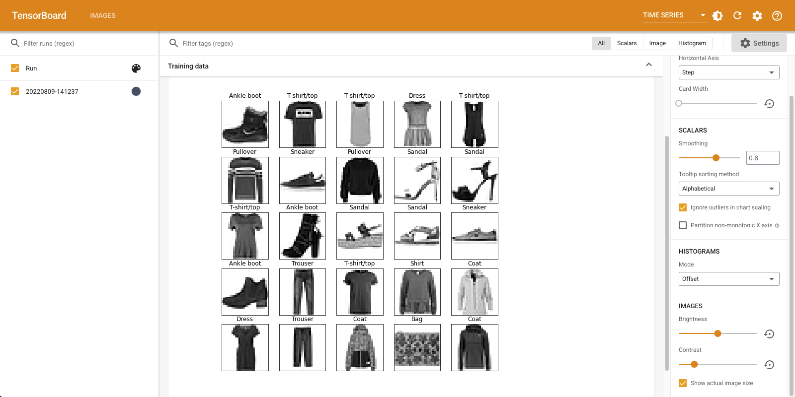
"छवियां" टैब उस छवि को प्रदर्शित करता है जिसे आपने अभी लॉग किया है। यह एक "टखने का बूट" है।
आसानी से देखने के लिए छवि को डिफ़ॉल्ट आकार में बढ़ाया जाता है। यदि आप बिना मापी गई मूल छवि देखना चाहते हैं, तो ऊपरी बाईं ओर "वास्तविक छवि आकार दिखाएं" चेक करें।
यह देखने के लिए कि वे छवि पिक्सेल को कैसे प्रभावित करते हैं, चमक और कंट्रास्ट स्लाइडर के साथ खेलें।
एकाधिक छवियों को विज़ुअलाइज़ करना
एक टेंसर को लॉग करना बहुत अच्छा है, लेकिन क्या होगा यदि आप कई प्रशिक्षण उदाहरणों को लॉग करना चाहते हैं?
सीधे शब्दों में आप जब करने के लिए डेटा गुजर प्रवेश करना चाहते हैं छवियों की संख्या निर्दिष्ट tf.summary.image() ।
with file_writer.as_default():
  # Don't forget to reshape.
  images = np.reshape(train_images[0:25], (-1, 28, 28, 1))
  tf.summary.image("25 training data examples", images, max_outputs=25, step=0)

%tensorboard --logdir logs/train_data

मनमाना छवि डेटा लॉगिंग
क्या होगा अगर आप इस तरह के द्वारा उत्पन्न एक छवि के रूप में एक छवि है कि एक टेन्सर नहीं है, कल्पना करने के लिए चाहते हैं matplotlib ?
प्लॉट को टेंसर में बदलने के लिए आपको कुछ बॉयलरप्लेट कोड की आवश्यकता होती है, लेकिन उसके बाद, आप जाने के लिए अच्छे हैं।
नीचे दिए गए कोड में, आप matplotlib का उपयोग एक अच्छा ग्रिड के रूप में पहले 25 छवियों प्रवेश करेंगे subplot() समारोह। फिर आप TensorBoard में ग्रिड देखेंगे:
# Clear out prior logging data.
!rm -rf logs/plots

logdir = "logs/plots/" + datetime.now().strftime("%Y%m%d-%H%M%S")
file_writer = tf.summary.create_file_writer(logdir)

def plot_to_image(figure):
  """Converts the matplotlib plot specified by 'figure' to a PNG image and
  returns it. The supplied figure is closed and inaccessible after this call."""
  # Save the plot to a PNG in memory.
  buf = io.BytesIO()
  plt.savefig(buf, format='png')
  # Closing the figure prevents it from being displayed directly inside
  # the notebook.
  plt.close(figure)
  buf.seek(0)
  # Convert PNG buffer to TF image
  image = tf.image.decode_png(buf.getvalue(), channels=4)
  # Add the batch dimension
  image = tf.expand_dims(image, 0)
  return image

def image_grid():
  """Return a 5x5 grid of the MNIST images as a matplotlib figure."""
  # Create a figure to contain the plot.
  figure = plt.figure(figsize=(10,10))
  for i in range(25):
    # Start next subplot.
    plt.subplot(5, 5, i + 1, title=class_names[train_labels[i]])
    plt.xticks([])
    plt.yticks([])
    plt.grid(False)
    plt.imshow(train_images[i], cmap=plt.cm.binary)

  return figure

# Prepare the plot
figure = image_grid()
# Convert to image and log
with file_writer.as_default():
  tf.summary.image("Training data", plot_to_image(figure), step=0)

%tensorboard --logdir logs/plots
इमेज क्लासिफायर का निर्माण
अब इस सब को एक वास्तविक उदाहरण के साथ एक साथ रखें। आखिरकार, आप यहां मशीन लर्निंग करने आए हैं, न कि सुंदर चित्र बनाने के लिए!
फैशन-एमएनआईएसटी डेटासेट के लिए एक साधारण क्लासिफायरियर को प्रशिक्षित करते समय आप यह समझने के लिए छवि सारांश का उपयोग करने जा रहे हैं कि आपका मॉडल कितना अच्छा कर रहा है।
सबसे पहले, एक बहुत ही सरल मॉडल बनाएं और इसे संकलित करें, ऑप्टिमाइज़र और लॉस फ़ंक्शन सेट करें। संकलन चरण यह भी निर्दिष्ट करता है कि आप रास्ते में क्लासिफायरियर की सटीकता को लॉग करना चाहते हैं।
model = keras.models.Sequential([
    keras.layers.Flatten(input_shape=(28, 28)),
    keras.layers.Dense(32, activation='relu'),
    keras.layers.Dense(10, activation='softmax')
])

model.compile(
    optimizer='adam',
    loss='sparse_categorical_crossentropy',
    metrics=['accuracy']
)
जब एक वर्गीकारक प्रशिक्षण, यह देखने के लिए उपयोगी है भ्रम मैट्रिक्स । कन्फ्यूजन मैट्रिक्स आपको विस्तृत जानकारी देता है कि आपका क्लासिफायरियर टेस्ट डेटा पर कैसा प्रदर्शन कर रहा है।
एक फ़ंक्शन को परिभाषित करें जो भ्रम मैट्रिक्स की गणना करता है। आप एक सुविधाजनक इस्तेमाल करेंगे Scikit सीखने समारोह ऐसा करने के लिए, और फिर matplotlib का उपयोग कर इसे साजिश।
def plot_confusion_matrix(cm, class_names):
  """
  Returns a matplotlib figure containing the plotted confusion matrix.

  Args:
    cm (array, shape = [n, n]): a confusion matrix of integer classes
    class_names (array, shape = [n]): String names of the integer classes
  """
  figure = plt.figure(figsize=(8, 8))
  plt.imshow(cm, interpolation='nearest', cmap=plt.cm.Blues)
  plt.title("Confusion matrix")
  plt.colorbar()
  tick_marks = np.arange(len(class_names))
  plt.xticks(tick_marks, class_names, rotation=45)
  plt.yticks(tick_marks, class_names)

  # Compute the labels from the normalized confusion matrix.
  labels = np.around(cm.astype('float') / cm.sum(axis=1)[:, np.newaxis], decimals=2)

  # Use white text if squares are dark; otherwise black.
  threshold = cm.max() / 2.
  for i, j in itertools.product(range(cm.shape[0]), range(cm.shape[1])):
    color = "white" if cm[i, j] > threshold else "black"
    plt.text(j, i, labels[i, j], horizontalalignment="center", color=color)

  plt.tight_layout()
  plt.ylabel('True label')
  plt.xlabel('Predicted label')
  return figure
अब आप क्लासिफायरियर को प्रशिक्षित करने के लिए तैयार हैं और रास्ते में नियमित रूप से भ्रम मैट्रिक्स को लॉग करते हैं।
यहाँ आप क्या करेंगे:
- बनाएं Keras TensorBoard कॉलबैक बुनियादी मीट्रिक लॉग इन करने के
- एक बनाएं Keras LambdaCallback हर युग के अंत में भ्रम की स्थिति मैट्रिक्स लॉग इन करने के
- Model.fit() का उपयोग करके मॉडल को प्रशिक्षित करें, दोनों कॉलबैक पास करना सुनिश्चित करें
जैसे-जैसे प्रशिक्षण आगे बढ़ता है, TensorBoard को प्रारंभ होते देखने के लिए नीचे स्क्रॉल करें।
# Clear out prior logging data.
!rm -rf logs/image

logdir = "logs/image/" + datetime.now().strftime("%Y%m%d-%H%M%S")
# Define the basic TensorBoard callback.
tensorboard_callback = keras.callbacks.TensorBoard(log_dir=logdir)
file_writer_cm = tf.summary.create_file_writer(logdir + '/cm')
def log_confusion_matrix(epoch, logs):
  # Use the model to predict the values from the validation dataset.
  test_pred_raw = model.predict(test_images)
  test_pred = np.argmax(test_pred_raw, axis=1)

  # Calculate the confusion matrix.
  cm = sklearn.metrics.confusion_matrix(test_labels, test_pred)
  # Log the confusion matrix as an image summary.
  figure = plot_confusion_matrix(cm, class_names=class_names)
  cm_image = plot_to_image(figure)

  # Log the confusion matrix as an image summary.
  with file_writer_cm.as_default():
    tf.summary.image("Confusion Matrix", cm_image, step=epoch)

# Define the per-epoch callback.
cm_callback = keras.callbacks.LambdaCallback(on_epoch_end=log_confusion_matrix)
# Start TensorBoard.
%tensorboard --logdir logs/image

# Train the classifier.
model.fit(
    train_images,
    train_labels,
    epochs=5,
    verbose=0, # Suppress chatty output
    callbacks=[tensorboard_callback, cm_callback],
    validation_data=(test_images, test_labels),
)
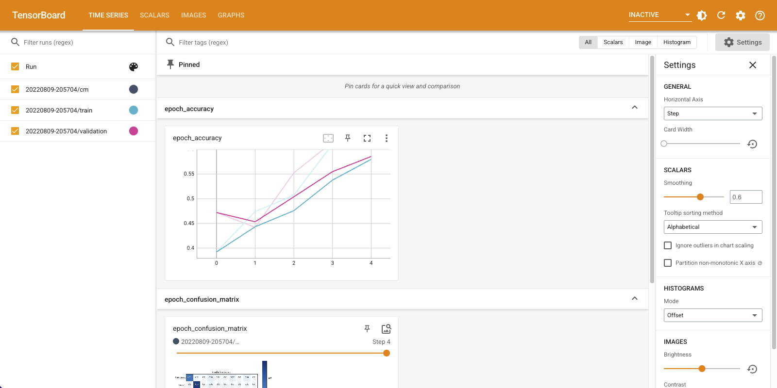
ध्यान दें कि सटीकता ट्रेन और सत्यापन सेट दोनों पर चढ़ रही है। यह एक अच्छा संकेत है। लेकिन मॉडल डेटा के विशिष्ट सबसेट पर कैसा प्रदर्शन कर रहा है?
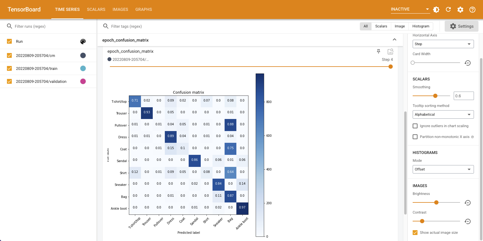
अपने लॉग किए गए कन्फ्यूजन मैट्रिसेस की कल्पना करने के लिए "इमेज" टैब चुनें। कन्फ्यूजन मैट्रिक्स को पूर्ण आकार में देखने के लिए ऊपर बाईं ओर "वास्तविक छवि आकार दिखाएं" चेक करें।
डिफ़ॉल्ट रूप से डैशबोर्ड अंतिम लॉग किए गए चरण या युग के लिए छवि सारांश दिखाता है। पहले के कन्फ्यूजन मैट्रिसेस देखने के लिए स्लाइडर का उपयोग करें। ध्यान दें कि जैसे-जैसे प्रशिक्षण आगे बढ़ता है, मैट्रिक्स में महत्वपूर्ण रूप से परिवर्तन होता है, विकर्ण के साथ गहरे वर्गों के साथ, और शेष मैट्रिक्स 0 और सफेद की ओर झुकता है। इसका मतलब है कि जैसे-जैसे प्रशिक्षण आगे बढ़ रहा है, आपका क्लासिफायरियर सुधर रहा है! महान काम!
भ्रम मैट्रिक्स से पता चलता है कि इस सरल मॉडल में कुछ समस्याएं हैं। बड़ी प्रगति के बावजूद, शर्ट, टी-शर्ट और पुलओवर एक दूसरे के साथ भ्रमित हो रहे हैं। मॉडल को और काम करने की जरूरत है।
आप रुचि रखते हैं, एक साथ इस मॉडल में सुधार की कोशिश convolutional नेटवर्क (सीएनएन)।