TensorFlow가 5월 14일 Google I/O로 돌아왔습니다! 지금 등록하세요

이 페이지는 Cloud Translation API를 통해 번역되었습니다.

TensorBoard에서 이미지 데이터 표시

개요

TensorFlow 이미지 요약 API를 사용하면 쉽게 텐서 및 임의의 이미지를 기록하고 TensorBoard에서 볼 수 있습니다. 이 샘플과 입력 데이터를 검사하거나 매우 도움이 될 수있는 계층 무게 시각화 및 생성 텐서를 . 모델 개발 과정에서 도움이 될 수 있는 이미지로 진단 데이터를 기록할 수도 있습니다.

이 튜토리얼에서는 이미지 요약 API를 사용하여 텐서를 이미지로 시각화하는 방법을 배웁니다. 또한 임의의 이미지를 가져와서 텐서로 변환하고 TensorBoard에서 시각화하는 방법을 배우게 됩니다. 모델의 성능을 이해하는 데 도움이 되도록 이미지 요약을 사용하는 간단하지만 실제적인 예를 통해 작업합니다.

설정

try:
  # %tensorflow_version only exists in Colab.
  %tensorflow_version 2.x
except Exception:
  pass

# Load the TensorBoard notebook extension.
%load_ext tensorboard

TensorFlow 2.x selected.

from datetime import datetime
import io
import itertools
from packaging import version

import tensorflow as tf
from tensorflow import keras

import matplotlib.pyplot as plt
import numpy as np
import sklearn.metrics

print("TensorFlow version: ", tf.__version__)
assert version.parse(tf.__version__).release[0] >= 2, \
    "This notebook requires TensorFlow 2.0 or above."

TensorFlow version:  2.2

Fashion-MNIST 데이터 세트 다운로드

당신은 상기의 분류 이미지에 간단한 신경 네트워크를 구성하는거야 패션 - MNIST의 데이터 세트. 이 데이터세트는 10개 카테고리의 패션 제품에 대한 70,000개의 28x28 그레이스케일 이미지로 구성되며 카테고리당 7,000개의 이미지가 있습니다.

먼저 데이터를 다운로드합니다.

# Download the data. The data is already divided into train and test.
# The labels are integers representing classes.
fashion_mnist = keras.datasets.fashion_mnist
(train_images, train_labels), (test_images, test_labels) = \
    fashion_mnist.load_data()

# Names of the integer classes, i.e., 0 -> T-short/top, 1 -> Trouser, etc.
class_names = ['T-shirt/top', 'Trouser', 'Pullover', 'Dress', 'Coat', 
    'Sandal', 'Shirt', 'Sneaker', 'Bag', 'Ankle boot']

Downloading data from https://storage.googleapis.com/tensorflow/tf-keras-datasets/train-labels-idx1-ubyte.gz
32768/29515 [=================================] - 0s 0us/step
Downloading data from https://storage.googleapis.com/tensorflow/tf-keras-datasets/train-images-idx3-ubyte.gz
26427392/26421880 [==============================] - 0s 0us/step
Downloading data from https://storage.googleapis.com/tensorflow/tf-keras-datasets/t10k-labels-idx1-ubyte.gz
8192/5148 [===============================================] - 0s 0us/step
Downloading data from https://storage.googleapis.com/tensorflow/tf-keras-datasets/t10k-images-idx3-ubyte.gz
4423680/4422102 [==============================] - 0s 0us/step

단일 이미지 시각화

Image Summary API의 작동 방식을 이해하기 위해 이제 TensorBoard에서 훈련 세트의 첫 번째 훈련 이미지를 간단히 기록할 것입니다.

그렇게 하기 전에 훈련 데이터의 모양을 검사하십시오.

print("Shape: ", train_images[0].shape)
print("Label: ", train_labels[0], "->", class_names[train_labels[0]])

Shape:  (28, 28)
Label:  9 -> Ankle boot

데이터 세트에 있는 각 이미지의 모양은 높이와 너비를 나타내는 모양(28, 28)의 랭크 2 텐서입니다.

그러나 tf.summary.image() 함유하는 등급 4 텐서 기대 (batch_size, height, width, channels) . 따라서 텐서를 재구성해야 합니다.

그래서 당신은 하나 개의 이미지,있는 거 로깅 batch_size 이미지는 그레이 스케일이다 1, 그래서 설정 channels 1로.

# Reshape the image for the Summary API.
img = np.reshape(train_images[0], (-1, 28, 28, 1))

이제 이 이미지를 기록하고 TensorBoard에서 볼 준비가 되었습니다.

# Clear out any prior log data.
!rm -rf logs

# Sets up a timestamped log directory.
logdir = "logs/train_data/" + datetime.now().strftime("%Y%m%d-%H%M%S")
# Creates a file writer for the log directory.
file_writer = tf.summary.create_file_writer(logdir)

# Using the file writer, log the reshaped image.
with file_writer.as_default():
  tf.summary.image("Training data", img, step=0)

이제 TensorBoard를 사용하여 이미지를 검사합니다. UI가 회전할 때까지 몇 초 동안 기다립니다.

%tensorboard --logdir logs/train_data

"이미지" 탭에는 방금 기록한 이미지가 표시됩니다. "앵클부츠"입니다.

이미지는 더 쉽게 볼 수 있도록 기본 크기로 조정됩니다. 크기가 조정되지 않은 원본 이미지를 보려면 왼쪽 상단의 "실제 이미지 크기 표시"를 선택하십시오.

밝기 및 대비 슬라이더를 사용하여 이미지 픽셀에 미치는 영향을 확인합니다.

여러 이미지 시각화

하나의 텐서를 로깅하는 것도 좋지만 여러 훈련 예제를 로깅하려면 어떻게 해야 할까요?

단순히 당신이 데이터를 전달할 때 기록 할 이미지의 수를 지정 tf.summary.image() .

with file_writer.as_default():
  # Don't forget to reshape.
  images = np.reshape(train_images[0:25], (-1, 28, 28, 1))
  tf.summary.image("25 training data examples", images, max_outputs=25, step=0)

%tensorboard --logdir logs/train_data

임의의 이미지 데이터 로깅

당신은에 의해 생성 된 이미지로 텐서 아니라 이미지를 시각화하고 싶다면 하기 matplotlib ?

플롯을 텐서로 변환하려면 상용구 코드가 필요하지만 그 후에는 계속할 수 있습니다.

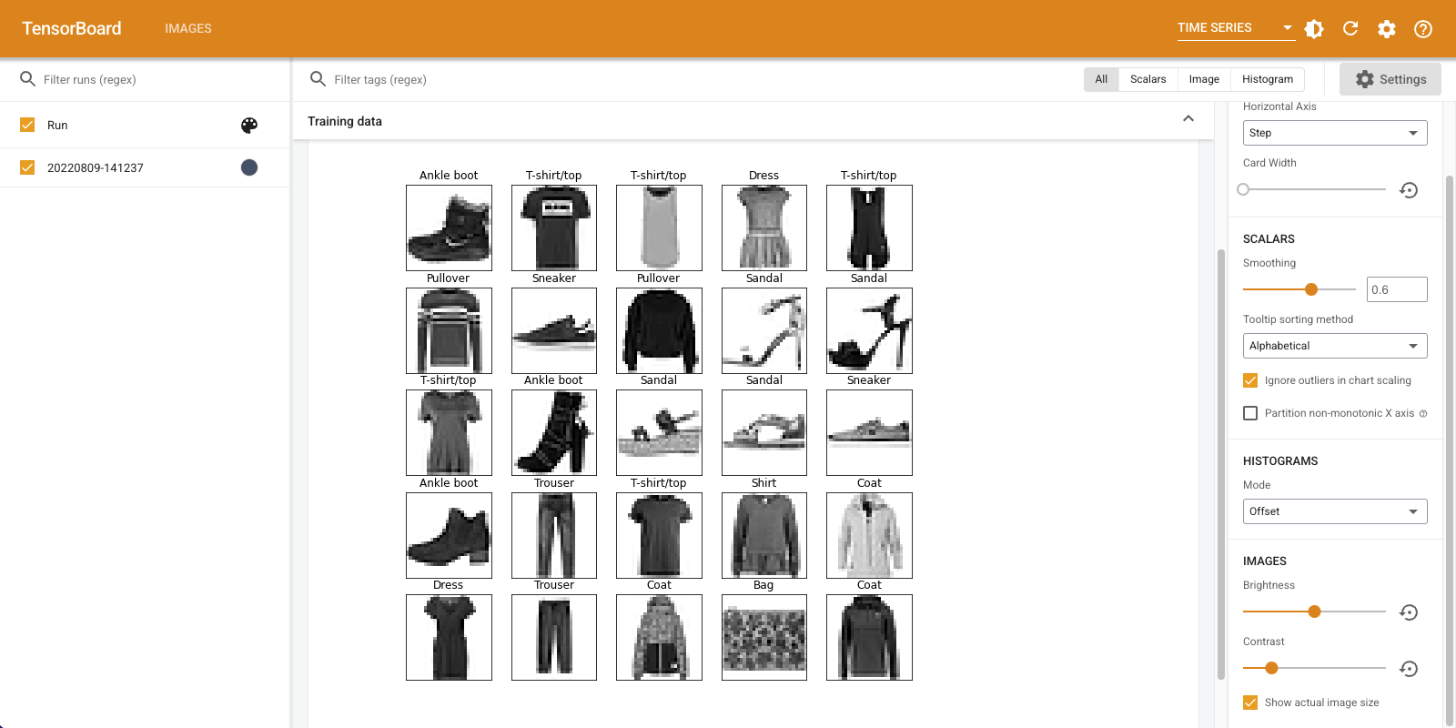
아래의 코드에서하기 matplotlib의 사용하여 좋은 그리드로 처음 25 개 이미지를 기록 할 것이다 subplot() 함수를. 그런 다음 TensorBoard에서 그리드를 볼 수 있습니다.

# Clear out prior logging data.
!rm -rf logs/plots

logdir = "logs/plots/" + datetime.now().strftime("%Y%m%d-%H%M%S")
file_writer = tf.summary.create_file_writer(logdir)

def plot_to_image(figure):
  """Converts the matplotlib plot specified by 'figure' to a PNG image and
  returns it. The supplied figure is closed and inaccessible after this call."""
  # Save the plot to a PNG in memory.
  buf = io.BytesIO()
  plt.savefig(buf, format='png')
  # Closing the figure prevents it from being displayed directly inside
  # the notebook.
  plt.close(figure)
  buf.seek(0)
  # Convert PNG buffer to TF image
  image = tf.image.decode_png(buf.getvalue(), channels=4)
  # Add the batch dimension
  image = tf.expand_dims(image, 0)
  return image

def image_grid():
  """Return a 5x5 grid of the MNIST images as a matplotlib figure."""
  # Create a figure to contain the plot.
  figure = plt.figure(figsize=(10,10))
  for i in range(25):
    # Start next subplot.
    plt.subplot(5, 5, i + 1, title=class_names[train_labels[i]])
    plt.xticks([])
    plt.yticks([])
    plt.grid(False)
    plt.imshow(train_images[i], cmap=plt.cm.binary)

  return figure

# Prepare the plot
figure = image_grid()
# Convert to image and log
with file_writer.as_default():
  tf.summary.image("Training data", plot_to_image(figure), step=0)

%tensorboard --logdir logs/plots

이미지 분류기 빌드

이제 이 모든 것을 실제 예와 함께 사용하십시오. 결국, 당신은 멋진 그림을 그리는 것이 아니라 기계 학습을 하기 위해 왔습니다!

Fashion-MNIST 데이터 세트에 대한 간단한 분류기를 훈련하는 동안 모델이 얼마나 잘 작동하는지 이해하기 위해 이미지 요약을 사용할 것입니다.

먼저 아주 간단한 모델을 만들고 컴파일하고 옵티마이저와 손실 함수를 설정합니다. 또한 컴파일 단계에서는 분류기의 정확도를 기록하도록 지정합니다.

model = keras.models.Sequential([
    keras.layers.Flatten(input_shape=(28, 28)),
    keras.layers.Dense(32, activation='relu'),
    keras.layers.Dense(10, activation='softmax')
])

model.compile(
    optimizer='adam', 
    loss='sparse_categorical_crossentropy',
    metrics=['accuracy']
)

분류기를 훈련 할 때, 볼 유용 혼동 행렬을 . 혼동 행렬은 분류기가 테스트 데이터에 대해 수행하는 방식에 대한 자세한 지식을 제공합니다.

정오분류표를 계산하는 함수를 정의합니다. 당신은 편리한 사용합니다 Scikit 배우기 이 작업을 수행하는 기능을하고하기 matplotlib를 사용하여 플롯.

def plot_confusion_matrix(cm, class_names):
  """
  Returns a matplotlib figure containing the plotted confusion matrix.

  Args:
    cm (array, shape = [n, n]): a confusion matrix of integer classes
    class_names (array, shape = [n]): String names of the integer classes
  """
  figure = plt.figure(figsize=(8, 8))
  plt.imshow(cm, interpolation='nearest', cmap=plt.cm.Blues)
  plt.title("Confusion matrix")
  plt.colorbar()
  tick_marks = np.arange(len(class_names))
  plt.xticks(tick_marks, class_names, rotation=45)
  plt.yticks(tick_marks, class_names)

  # Compute the labels from the normalized confusion matrix.
  labels = np.around(cm.astype('float') / cm.sum(axis=1)[:, np.newaxis], decimals=2)

  # Use white text if squares are dark; otherwise black.
  threshold = cm.max() / 2.
  for i, j in itertools.product(range(cm.shape[0]), range(cm.shape[1])):
    color = "white" if cm[i, j] > threshold else "black"
    plt.text(j, i, labels[i, j], horizontalalignment="center", color=color)

  plt.tight_layout()
  plt.ylabel('True label')
  plt.xlabel('Predicted label')
  return figure

이제 분류기를 훈련하고 그 과정에서 정오분류표를 정기적으로 기록할 준비가 되었습니다.

수행할 작업은 다음과 같습니다.

만들기 Keras TensorBoard 콜백 기본 통계를 기록하기를
크리에이트 Keras LambdaCallback을 모든 시대의 끝에서 혼란 매트릭스를 기록
Model.fit()을 사용하여 모델을 훈련하고 두 콜백을 모두 전달해야 합니다.

교육이 진행되면 아래로 스크롤하여 TensorBoard가 시작되는 것을 확인합니다.

# Clear out prior logging data.
!rm -rf logs/image

logdir = "logs/image/" + datetime.now().strftime("%Y%m%d-%H%M%S")
# Define the basic TensorBoard callback.
tensorboard_callback = keras.callbacks.TensorBoard(log_dir=logdir)
file_writer_cm = tf.summary.create_file_writer(logdir + '/cm')

def log_confusion_matrix(epoch, logs):
  # Use the model to predict the values from the validation dataset.
  test_pred_raw = model.predict(test_images)
  test_pred = np.argmax(test_pred_raw, axis=1)

  # Calculate the confusion matrix.
  cm = sklearn.metrics.confusion_matrix(test_labels, test_pred)
  # Log the confusion matrix as an image summary.
  figure = plot_confusion_matrix(cm, class_names=class_names)
  cm_image = plot_to_image(figure)

  # Log the confusion matrix as an image summary.
  with file_writer_cm.as_default():
    tf.summary.image("Confusion Matrix", cm_image, step=epoch)

# Define the per-epoch callback.
cm_callback = keras.callbacks.LambdaCallback(on_epoch_end=log_confusion_matrix)

# Start TensorBoard.
%tensorboard --logdir logs/image

# Train the classifier.
model.fit(
    train_images,
    train_labels,
    epochs=5,
    verbose=0, # Suppress chatty output
    callbacks=[tensorboard_callback, cm_callback],
    validation_data=(test_images, test_labels),
)

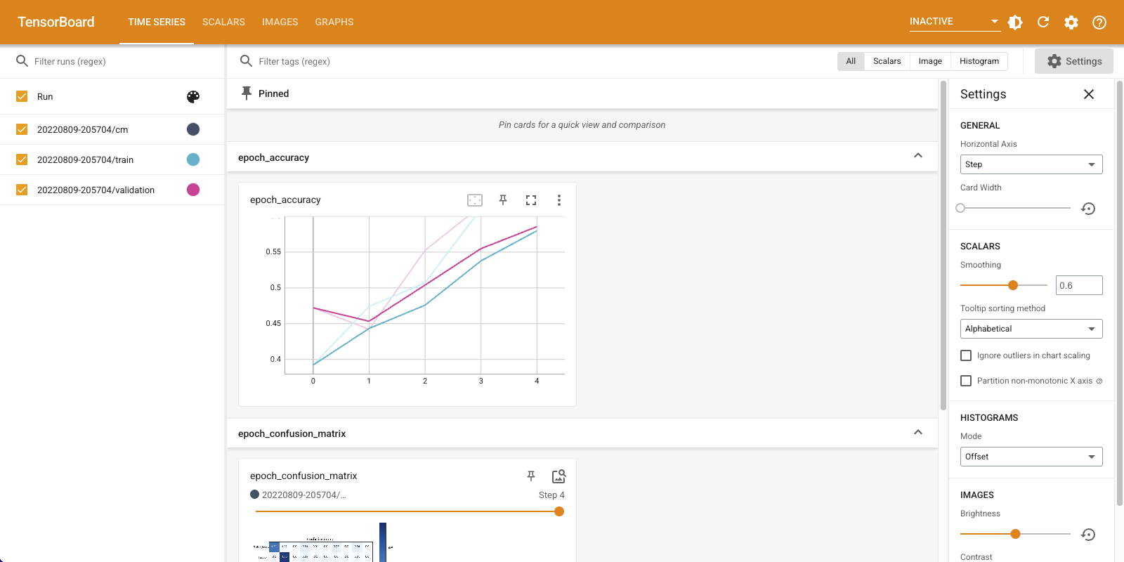
정확도는 기차와 검증 세트 모두에서 증가하고 있습니다. 좋은 징조입니다. 그러나 모델은 데이터의 특정 하위 집합에서 어떻게 수행됩니까?

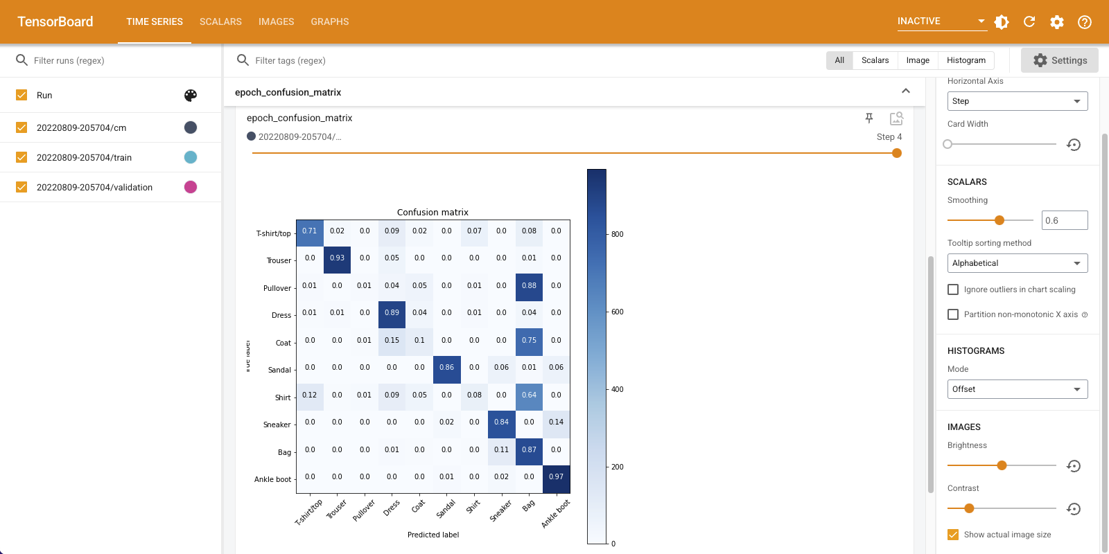
기록된 혼동 매트릭스를 시각화하려면 "이미지" 탭을 선택하십시오. 전체 크기로 혼동 행렬을 보려면 왼쪽 상단의 "실제 이미지 크기 표시"를 선택하십시오.

기본적으로 대시보드에는 마지막으로 기록된 단계 또는 에포크에 대한 이미지 요약이 표시됩니다. 슬라이더를 사용하여 이전 혼동 행렬을 봅니다. 더 어두운 사각형이 대각선을 따라 합쳐지고 나머지 행렬이 0과 흰색을 향하는 경향이 있어 훈련이 진행됨에 따라 행렬이 어떻게 크게 변하는지 주목하십시오. 이것은 훈련이 진행됨에 따라 분류기가 향상되고 있음을 의미합니다! 훌륭한 일!

혼동 행렬은 이 간단한 모델에 몇 가지 문제가 있음을 보여줍니다. 큰 발전에도 불구하고 셔츠, 티셔츠, 풀오버는 서로 혼동되고 있습니다. 모델은 더 많은 작업이 필요합니다.

당신이 관심이 경우이 모델 개선하려고 길쌈 네트워크 (CNN)를.