
| |
|
 在 GitHub 上查看源代码 在 GitHub 上查看源代码 |
|
本教程展示了如何训练一个简单的卷积神经网络 (CNN) 来对 CIFAR 图像进行分类。由于本教程使用的是 Keras Sequential API,创建和训练模型只需要几行代码。
导入 TensorFlow
import tensorflow as tf

from tensorflow.keras import datasets, layers, models
import matplotlib.pyplot as plt
2023-11-07 23:07:35.116262: E external/local_xla/xla/stream_executor/cuda/cuda_dnn.cc:9261] Unable to register cuDNN factory: Attempting to register factory for plugin cuDNN when one has already been registered
2023-11-07 23:07:35.116317: E external/local_xla/xla/stream_executor/cuda/cuda_fft.cc:607] Unable to register cuFFT factory: Attempting to register factory for plugin cuFFT when one has already been registered
2023-11-07 23:07:35.118021: E external/local_xla/xla/stream_executor/cuda/cuda_blas.cc:1515] Unable to register cuBLAS factory: Attempting to register factory for plugin cuBLAS when one has already been registered
下载并准备 CIFAR10 数据集
CIFAR10 数据集包含 10 类,共 60000 张彩色图片,每类图片有 6000 张。此数据集中 50000 个样例被作为训练集,剩余 10000 个样例作为测试集。类之间相互独立,不存在重叠的部分。
(train_images, train_labels), (test_images, test_labels) = datasets.cifar10.load_data()

# Normalize pixel values to be between 0 and 1
train_images, test_images = train_images / 255.0, test_images / 255.0
Downloading data from https://www.cs.toronto.edu/~kriz/cifar-10-python.tar.gz
170498071/170498071 [==============================] - 2s 0us/step
验证数据
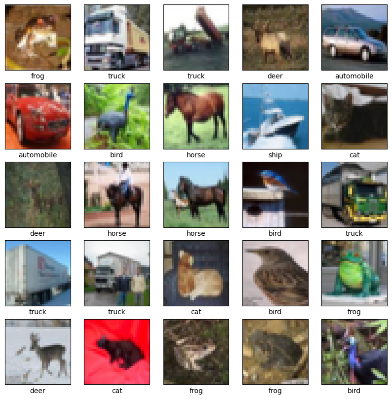
为了验证数据集看起来是否正确,我们绘制训练集中的前 25 张图像并在每张图像下方显示类名称:
class_names = ['airplane', 'automobile', 'bird', 'cat', 'deer',
               'dog', 'frog', 'horse', 'ship', 'truck']

plt.figure(figsize=(10,10))
for i in range(25):
    plt.subplot(5,5,i+1)
    plt.xticks([])
    plt.yticks([])
    plt.grid(False)
    plt.imshow(train_images[i])
    # The CIFAR labels happen to be arrays,
    # which is why you need the extra index
    plt.xlabel(class_names[train_labels[i][0]])
plt.show()
构造卷积神经网络模型
下方展示的 6 行代码声明了了一个常见卷积神经网络,由几个 Conv2D 和 MaxPooling2D 层组成。
CNN 将形状为 (image_height, image_width, color_channels) 的张量作为输入,忽略批次大小。如果您不熟悉这些维度,color_channels 是指 (R,G,B)。在此示例中,您将配置 CNN 以处理形状为 (32, 32, 3) 的输入,即 CIFAR 图像的格式。您可以通过将参数 input_shape 传递给第一层来实现此目的。
model = models.Sequential()
model.add(layers.Conv2D(32, (3, 3), activation='relu', input_shape=(32, 32, 3)))
model.add(layers.MaxPooling2D((2, 2)))
model.add(layers.Conv2D(64, (3, 3), activation='relu'))
model.add(layers.MaxPooling2D((2, 2)))
model.add(layers.Conv2D(64, (3, 3), activation='relu'))
到目前为止,模型的架构如下:
model.summary()
Model: "sequential"
_________________________________________________________________
 Layer (type)                Output Shape              Param #
=================================================================
 conv2d (Conv2D)             (None, 30, 30, 32)        896

 max_pooling2d (MaxPooling2  (None, 15, 15, 32)        0
 D)

 conv2d_1 (Conv2D)           (None, 13, 13, 64)        18496

 max_pooling2d_1 (MaxPoolin  (None, 6, 6, 64)          0
 g2D)

 conv2d_2 (Conv2D)           (None, 4, 4, 64)          36928

=================================================================
Total params: 56320 (220.00 KB)
Trainable params: 56320 (220.00 KB)
Non-trainable params: 0 (0.00 Byte)
_________________________________________________________________
在上面的结构中,您可以看到每个 Conv2D 和 MaxPooling2D 层的输出都是一个三维的张量 (Tensor),其形状描述了 (height, width, channels)。越深的层中,宽度和高度都会收缩。每个 Conv2D 层输出的通道数量 (channels) 取决于声明层时的第一个参数(如:上面代码中的 32 或 64)。这样,由于宽度和高度的收缩,您便可以(从运算的角度)增加每个 Conv2D 层输出的通道数量 (channels)。
增加 Dense 层
为了完成模型,您需要将卷积基(形状为 (4, 4, 64))的最后一个输出张量馈送到一个或多个 Dense 层以执行分类。Dense 层将向量作为输入(即 1 维),而当前输出为 3 维张量。首先,将 3 维输出展平(或展开)为 1 维,然后在顶部添加一个或多个 Dense 层。CIFAR 有 10 个输出类,因此使用具有 10 个输出的最终 Dense 层。
model.add(layers.Flatten())
model.add(layers.Dense(64, activation='relu'))
model.add(layers.Dense(10))
下面是模型的完整架构:
model.summary()
Model: "sequential"
_________________________________________________________________
 Layer (type)                Output Shape              Param #
=================================================================
 conv2d (Conv2D)             (None, 30, 30, 32)        896

 max_pooling2d (MaxPooling2  (None, 15, 15, 32)        0
 D)

 conv2d_1 (Conv2D)           (None, 13, 13, 64)        18496

 max_pooling2d_1 (MaxPoolin  (None, 6, 6, 64)          0
 g2D)

 conv2d_2 (Conv2D)           (None, 4, 4, 64)          36928

 flatten (Flatten)           (None, 1024)              0

 dense (Dense)               (None, 64)                65600

 dense_1 (Dense)             (None, 10)                650

=================================================================
Total params: 122570 (478.79 KB)
Trainable params: 122570 (478.79 KB)
Non-trainable params: 0 (0.00 Byte)
_________________________________________________________________
网络摘要显示 (4, 4, 64) 输出在经过两个 Dense 层之前被展平为形状为 (1024) 的向量。
编译并训练模型
model.compile(optimizer='adam',
              loss=tf.keras.losses.SparseCategoricalCrossentropy(from_logits=True),
              metrics=['accuracy'])

history = model.fit(train_images, train_labels, epochs=10,
                    validation_data=(test_images, test_labels))
Epoch 1/10
WARNING: All log messages before absl::InitializeLog() is called are written to STDERR
I0000 00:00:1699398471.661645  508357 device_compiler.h:186] Compiled cluster using XLA!  This line is logged at most once for the lifetime of the process.
1563/1563 [==============================] - 11s 5ms/step - loss: 1.5134 - accuracy: 0.4460 - val_loss: 1.2960 - val_accuracy: 0.5345
Epoch 2/10
1563/1563 [==============================] - 7s 4ms/step - loss: 1.1488 - accuracy: 0.5939 - val_loss: 1.0667 - val_accuracy: 0.6218
Epoch 3/10
1563/1563 [==============================] - 7s 4ms/step - loss: 1.0076 - accuracy: 0.6447 - val_loss: 1.0151 - val_accuracy: 0.6442
Epoch 4/10
1563/1563 [==============================] - 7s 4ms/step - loss: 0.9155 - accuracy: 0.6785 - val_loss: 0.9411 - val_accuracy: 0.6718
Epoch 5/10
1563/1563 [==============================] - 7s 4ms/step - loss: 0.8463 - accuracy: 0.7040 - val_loss: 0.9239 - val_accuracy: 0.6766
Epoch 6/10
1563/1563 [==============================] - 7s 4ms/step - loss: 0.7910 - accuracy: 0.7224 - val_loss: 0.9261 - val_accuracy: 0.6806
Epoch 7/10
1563/1563 [==============================] - 7s 4ms/step - loss: 0.7454 - accuracy: 0.7389 - val_loss: 0.9613 - val_accuracy: 0.6720
Epoch 8/10
1563/1563 [==============================] - 7s 4ms/step - loss: 0.7033 - accuracy: 0.7546 - val_loss: 0.9221 - val_accuracy: 0.6836
Epoch 9/10
1563/1563 [==============================] - 7s 4ms/step - loss: 0.6627 - accuracy: 0.7662 - val_loss: 0.8851 - val_accuracy: 0.6999
Epoch 10/10
1563/1563 [==============================] - 7s 4ms/step - loss: 0.6279 - accuracy: 0.7790 - val_loss: 0.9152 - val_accuracy: 0.6958
评估模型
plt.plot(history.history['accuracy'], label='accuracy')
plt.plot(history.history['val_accuracy'], label = 'val_accuracy')
plt.xlabel('Epoch')
plt.ylabel('Accuracy')
plt.ylim([0.5, 1])
plt.legend(loc='lower right')

test_loss, test_acc = model.evaluate(test_images,  test_labels, verbose=2)
313/313 - 1s - loss: 0.9152 - accuracy: 0.6958 - 670ms/epoch - 2ms/step
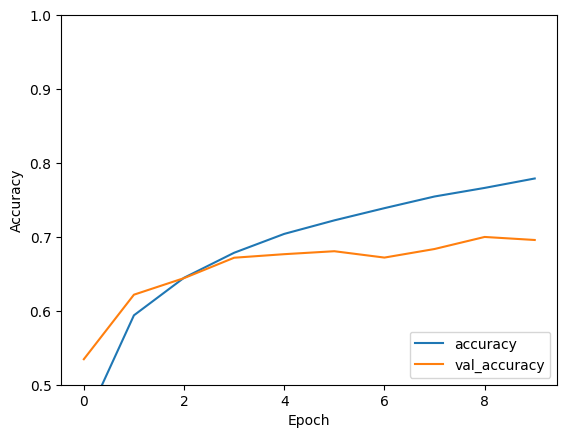
print(test_acc)
0.6958000063896179
您的简单 CNN 的测试准确率已达到 70% 以上。对于只有几行的代码来说,效果不错!对于另一种 CNN 风格,请参阅适合专家的 TensorFlow 2 快速入门示例,此示例使用了 Keras 子类化 API 和 tf.GradientTape。