يوضح هذا الكمبيوتر الدفتري مثالين لملاءمة نماذج السلاسل الزمنية الهيكلية مع السلاسل الزمنية واستخدامها لتوليد التنبؤات والتفسيرات.
| | |  عرض المصدر على جيثب عرض المصدر على جيثب | |
التبعيات والمتطلبات
الاستيراد والإعداد
%matplotlib inline
import matplotlib as mpl
from matplotlib import pylab as plt
import matplotlib.dates as mdates
import seaborn as sns

import collections

import numpy as np
import tensorflow.compat.v2 as tf
import tensorflow_probability as tfp

from tensorflow_probability import distributions as tfd
from tensorflow_probability import sts

tf.enable_v2_behavior()
اجعل الأمور سريعة!
قبل أن نتعمق ، دعنا نتأكد من أننا نستخدم وحدة معالجة الرسومات لهذا العرض التوضيحي.
للقيام بذلك ، حدد "وقت التشغيل" -> "تغيير نوع وقت التشغيل" -> "مسرع الأجهزة" -> "GPU".
سيتحقق المقتطف التالي من أن لدينا حق الوصول إلى وحدة معالجة الرسومات.
if tf.test.gpu_device_name() != '/device:GPU:0':
  print('WARNING: GPU device not found.')
else:
  print('SUCCESS: Found GPU: {}'.format(tf.test.gpu_device_name()))
SUCCESS: Found GPU: /device:GPU:0
الإعداد التآمر
الطرق المساعدة لرسم السلاسل الزمنية والتنبؤات.
from pandas.plotting import register_matplotlib_converters
register_matplotlib_converters()

sns.set_context("notebook", font_scale=1.)
sns.set_style("whitegrid")
%config InlineBackend.figure_format = 'retina'
def plot_forecast(x, y,
                  forecast_mean, forecast_scale, forecast_samples,
                  title, x_locator=None, x_formatter=None):
  """Plot a forecast distribution against the 'true' time series."""
  colors = sns.color_palette()
  c1, c2 = colors[0], colors[1]
  fig = plt.figure(figsize=(12, 6))
  ax = fig.add_subplot(1, 1, 1)

  num_steps = len(y)
  num_steps_forecast = forecast_mean.shape[-1]
  num_steps_train = num_steps - num_steps_forecast


  ax.plot(x, y, lw=2, color=c1, label='ground truth')

  forecast_steps = np.arange(
      x[num_steps_train],
      x[num_steps_train]+num_steps_forecast,
      dtype=x.dtype)

  ax.plot(forecast_steps, forecast_samples.T, lw=1, color=c2, alpha=0.1)

  ax.plot(forecast_steps, forecast_mean, lw=2, ls='--', color=c2,
           label='forecast')
  ax.fill_between(forecast_steps,
                   forecast_mean-2*forecast_scale,
                   forecast_mean+2*forecast_scale, color=c2, alpha=0.2)

  ymin, ymax = min(np.min(forecast_samples), np.min(y)), max(np.max(forecast_samples), np.max(y))
  yrange = ymax-ymin
  ax.set_ylim([ymin - yrange*0.1, ymax + yrange*0.1])
  ax.set_title("{}".format(title))
  ax.legend()

  if x_locator is not None:
    ax.xaxis.set_major_locator(x_locator)
    ax.xaxis.set_major_formatter(x_formatter)
    fig.autofmt_xdate()

  return fig, ax
def plot_components(dates,
                    component_means_dict,
                    component_stddevs_dict,
                    x_locator=None,
                    x_formatter=None):
  """Plot the contributions of posterior components in a single figure."""
  colors = sns.color_palette()
  c1, c2 = colors[0], colors[1]

  axes_dict = collections.OrderedDict()
  num_components = len(component_means_dict)
  fig = plt.figure(figsize=(12, 2.5 * num_components))
  for i, component_name in enumerate(component_means_dict.keys()):
    component_mean = component_means_dict[component_name]
    component_stddev = component_stddevs_dict[component_name]

    ax = fig.add_subplot(num_components,1,1+i)
    ax.plot(dates, component_mean, lw=2)
    ax.fill_between(dates,
                     component_mean-2*component_stddev,
                     component_mean+2*component_stddev,
                     color=c2, alpha=0.5)
    ax.set_title(component_name)
    if x_locator is not None:
      ax.xaxis.set_major_locator(x_locator)
      ax.xaxis.set_major_formatter(x_formatter)
    axes_dict[component_name] = ax
  fig.autofmt_xdate()
  fig.tight_layout()
  return fig, axes_dict
def plot_one_step_predictive(dates, observed_time_series,
                             one_step_mean, one_step_scale,
                             x_locator=None, x_formatter=None):
  """Plot a time series against a model's one-step predictions."""

  colors = sns.color_palette()
  c1, c2 = colors[0], colors[1]

  fig=plt.figure(figsize=(12, 6))
  ax = fig.add_subplot(1,1,1)
  num_timesteps = one_step_mean.shape[-1]
  ax.plot(dates, observed_time_series, label="observed time series", color=c1)
  ax.plot(dates, one_step_mean, label="one-step prediction", color=c2)
  ax.fill_between(dates,
                  one_step_mean - one_step_scale,
                  one_step_mean + one_step_scale,
                  alpha=0.1, color=c2)
  ax.legend()

  if x_locator is not None:
    ax.xaxis.set_major_locator(x_locator)
    ax.xaxis.set_major_formatter(x_formatter)
    fig.autofmt_xdate()
  fig.tight_layout()
  return fig, ax
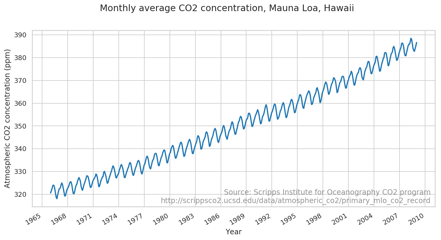
سجل Mauna Loa CO2
سنعرض نموذجًا ملائمًا لقراءات ثاني أكسيد الكربون في الغلاف الجوي من مرصد ماونا لوا.
البيانات
# CO2 readings from Mauna Loa observatory, monthly beginning January 1966
# Original source: http://scrippsco2.ucsd.edu/data/atmospheric_co2/primary_mlo_co2_record
co2_by_month = np.array('320.62,321.60,322.39,323.70,324.08,323.75,322.38,320.36,318.64,318.10,319.78,321.03,322.33,322.50,323.04,324.42,325.00,324.09,322.54,320.92,319.25,319.39,320.73,321.96,322.57,323.15,323.89,325.02,325.57,325.36,324.14,322.11,320.33,320.25,321.32,322.89,324.00,324.42,325.63,326.66,327.38,326.71,325.88,323.66,322.38,321.78,322.85,324.12,325.06,325.98,326.93,328.14,328.08,327.67,326.34,324.69,323.10,323.06,324.01,325.13,326.17,326.68,327.17,327.79,328.92,328.57,327.36,325.43,323.36,323.56,324.80,326.01,326.77,327.63,327.75,329.73,330.07,329.09,328.04,326.32,324.84,325.20,326.50,327.55,328.55,329.56,330.30,331.50,332.48,332.07,330.87,329.31,327.51,327.18,328.16,328.64,329.35,330.71,331.48,332.65,333.09,332.25,331.18,329.39,327.43,327.37,328.46,329.57,330.40,331.40,332.04,333.31,333.97,333.60,331.90,330.06,328.56,328.34,329.49,330.76,331.75,332.56,333.50,334.58,334.88,334.33,333.05,330.94,329.30,328.94,330.31,331.68,332.93,333.42,334.70,336.07,336.75,336.27,334.92,332.75,331.59,331.16,332.40,333.85,334.97,335.38,336.64,337.76,338.01,337.89,336.54,334.68,332.76,332.55,333.92,334.95,336.23,336.76,337.96,338.88,339.47,339.29,337.73,336.09,333.92,333.86,335.29,336.73,338.01,338.36,340.07,340.77,341.47,341.17,339.56,337.60,335.88,336.02,337.10,338.21,339.24,340.48,341.38,342.51,342.91,342.25,340.49,338.43,336.69,336.86,338.36,339.61,340.75,341.61,342.70,343.57,344.14,343.35,342.06,339.81,337.98,337.86,339.26,340.49,341.38,342.52,343.10,344.94,345.76,345.32,343.98,342.38,339.87,339.99,341.15,342.99,343.70,344.50,345.28,347.06,347.43,346.80,345.39,343.28,341.07,341.35,342.98,344.22,344.97,345.99,347.42,348.35,348.93,348.25,346.56,344.67,343.09,342.80,344.24,345.56,346.30,346.95,347.85,349.55,350.21,349.55,347.94,345.90,344.85,344.17,345.66,346.90,348.02,348.48,349.42,350.99,351.85,351.26,349.51,348.10,346.45,346.36,347.81,348.96,350.43,351.73,352.22,353.59,354.22,353.79,352.38,350.43,348.73,348.88,350.07,351.34,352.76,353.07,353.68,355.42,355.67,355.12,353.90,351.67,349.80,349.99,351.30,352.52,353.66,354.70,355.38,356.20,357.16,356.23,354.81,352.91,350.96,351.18,352.83,354.21,354.72,355.75,357.16,358.60,359.34,358.24,356.17,354.02,352.15,352.21,353.75,354.99,355.99,356.72,357.81,359.15,359.66,359.25,357.02,355.00,353.01,353.31,354.16,355.40,356.70,357.17,358.38,359.46,360.28,359.60,357.57,355.52,353.69,353.99,355.34,356.80,358.37,358.91,359.97,361.26,361.69,360.94,359.55,357.48,355.84,356.00,357.58,359.04,359.97,361.00,361.64,363.45,363.80,363.26,361.89,359.45,358.05,357.75,359.56,360.70,362.05,363.24,364.02,364.71,365.41,364.97,363.65,361.48,359.45,359.61,360.76,362.33,363.18,363.99,364.56,366.36,366.80,365.63,364.47,362.50,360.19,360.78,362.43,364.28,365.33,366.15,367.31,368.61,369.30,368.88,367.64,365.78,363.90,364.23,365.46,366.97,368.15,368.87,369.59,371.14,371.00,370.35,369.27,366.93,364.64,365.13,366.68,368.00,369.14,369.46,370.51,371.66,371.83,371.69,370.12,368.12,366.62,366.73,368.29,369.53,370.28,371.50,372.12,372.86,374.02,373.31,371.62,369.55,367.96,368.09,369.68,371.24,372.44,373.08,373.52,374.85,375.55,375.40,374.02,371.48,370.70,370.25,372.08,373.78,374.68,375.62,376.11,377.65,378.35,378.13,376.61,374.48,372.98,373.00,374.35,375.69,376.79,377.36,378.39,380.50,380.62,379.55,377.76,375.83,374.05,374.22,375.84,377.44,378.34,379.61,380.08,382.05,382.24,382.08,380.67,378.67,376.42,376.80,378.31,379.96,381.37,382.02,382.56,384.37,384.92,384.03,382.28,380.48,378.81,379.06,380.14,381.66,382.58,383.71,384.34,386.23,386.41,385.87,384.45,381.84,380.86,380.86,382.36,383.61,385.07,385.84,385.83,386.77,388.51,388.05,386.25,384.08,383.09,382.78,384.01,385.11,386.65,387.12,388.52,389.57,390.16,389.62,388.07,386.08,384.65,384.33,386.05,387.49,388.55,390.07,391.01,392.38,393.22,392.24,390.33,388.52,386.84,387.16,388.67,389.81,391.30,391.92,392.45,393.37,394.28,393.69,392.59,390.21,389.00,388.93,390.24,391.80,393.07,393.35,394.36,396.43,396.87,395.88,394.52,392.54,391.13,391.01,392.95,394.34,395.61,396.85,397.26,398.35,399.98,398.87,397.37,395.41,393.39,393.70,395.19,396.82,397.92,398.10,399.47,401.33,401.88,401.31,399.07,397.21,395.40,395.65,397.23,398.79,399.85,400.31,401.51,403.45,404.10,402.88,401.61,399.00,397.50,398.28,400.24,401.89,402.65,404.16,404.85,407.57,407.66,407.00,404.50,402.24,401.01,401.50,403.64,404.55,406.07,406.64,407.06,408.95,409.91,409.12,407.20,405.24,403.27,403.64,405.17,406.75,408.05,408.34,409.25,410.30,411.30,410.88,408.90,407.10,405.59,405.99,408.12,409.23,410.92'.split(',')).astype(np.float32)

co2_by_month = co2_by_month
num_forecast_steps = 12 * 10 # Forecast the final ten years, given previous data
co2_by_month_training_data = co2_by_month[:-num_forecast_steps]

co2_dates = np.arange("1966-01", "2019-02", dtype="datetime64[M]")
co2_loc = mdates.YearLocator(3)
co2_fmt = mdates.DateFormatter('%Y')
fig = plt.figure(figsize=(12, 6))
ax = fig.add_subplot(1, 1, 1)
ax.plot(co2_dates[:-num_forecast_steps], co2_by_month_training_data, lw=2, label="training data")
ax.xaxis.set_major_locator(co2_loc)
ax.xaxis.set_major_formatter(co2_fmt)
ax.set_ylabel("Atmospheric CO2 concentration (ppm)")
ax.set_xlabel("Year")
fig.suptitle("Monthly average CO2 concentration, Mauna Loa, Hawaii",
             fontsize=15)
ax.text(0.99, .02,
        "Source: Scripps Institute for Oceanography CO2 program\nhttp://scrippsco2.ucsd.edu/data/atmospheric_co2/primary_mlo_co2_record",
        transform=ax.transAxes,
        horizontalalignment="right",
        alpha=0.5)
fig.autofmt_xdate()
النموذج والتركيب
سنصمم هذه السلسلة باستخدام اتجاه خطي محلي ، بالإضافة إلى التأثير الموسمي لشهر من العام.
def build_model(observed_time_series):
  trend = sts.LocalLinearTrend(observed_time_series=observed_time_series)
  seasonal = tfp.sts.Seasonal(
      num_seasons=12, observed_time_series=observed_time_series)
  model = sts.Sum([trend, seasonal], observed_time_series=observed_time_series)
  return model
سنلائم النموذج باستخدام الاستدلال المتغير. يتضمن ذلك تشغيل مُحسِّن لتقليل دالة الخسارة المتغيرة ، والحد الأدنى للأدلة السلبية (ELBO). يناسب هذا مجموعة من التوزيعات اللاحقة التقريبية للمعلمات (في الممارسة العملية ، نفترض أن هذه هي معايير مستقلة تم تحويلها إلى مساحة الدعم لكل معلمة).
تتطلب طرق التنبؤ tfp.sts عينات لاحقة كمدخلات ، لذلك سننتهي من خلال رسم مجموعة من العينات من المتغير الخلفي.
co2_model = build_model(co2_by_month_training_data)

# Build the variational surrogate posteriors `qs`.
variational_posteriors = tfp.sts.build_factored_surrogate_posterior(
    model=co2_model)
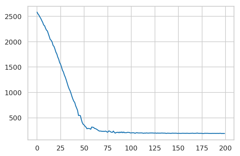
تقليل الخسارة المتغيرة.
# Allow external control of optimization to reduce test runtimes.
num_variational_steps = 200 # @param { isTemplate: true}
num_variational_steps = int(num_variational_steps)

# Build and optimize the variational loss function.
elbo_loss_curve = tfp.vi.fit_surrogate_posterior(
    target_log_prob_fn=co2_model.joint_distribution(
        observed_time_series=co2_by_month_training_data).log_prob,
    surrogate_posterior=variational_posteriors,
    optimizer=tf.optimizers.Adam(learning_rate=0.1),
    num_steps=num_variational_steps,
    jit_compile=True)

plt.plot(elbo_loss_curve)
plt.show()

# Draw samples from the variational posterior.
q_samples_co2_ = variational_posteriors.sample(50)
WARNING:tensorflow:From /usr/local/lib/python3.6/dist-packages/tensorflow_core/python/ops/linalg/linear_operator_diag.py:166: calling LinearOperator.__init__ (from tensorflow.python.ops.linalg.linear_operator) with graph_parents is deprecated and will be removed in a future version.
Instructions for updating:
Do not pass `graph_parents`.  They will  no longer be used.
print("Inferred parameters:")
for param in co2_model.parameters:
  print("{}: {} +- {}".format(param.name,
                              np.mean(q_samples_co2_[param.name], axis=0),
                              np.std(q_samples_co2_[param.name], axis=0)))
Inferred parameters:
observation_noise_scale: 0.17199112474918365 +- 0.009443143382668495
LocalLinearTrend/_level_scale: 0.17671072483062744 +- 0.01510554924607277
LocalLinearTrend/_slope_scale: 0.004302256740629673 +- 0.0018349259626120329
Seasonal/_drift_scale: 0.041069451719522476 +- 0.007772190496325493
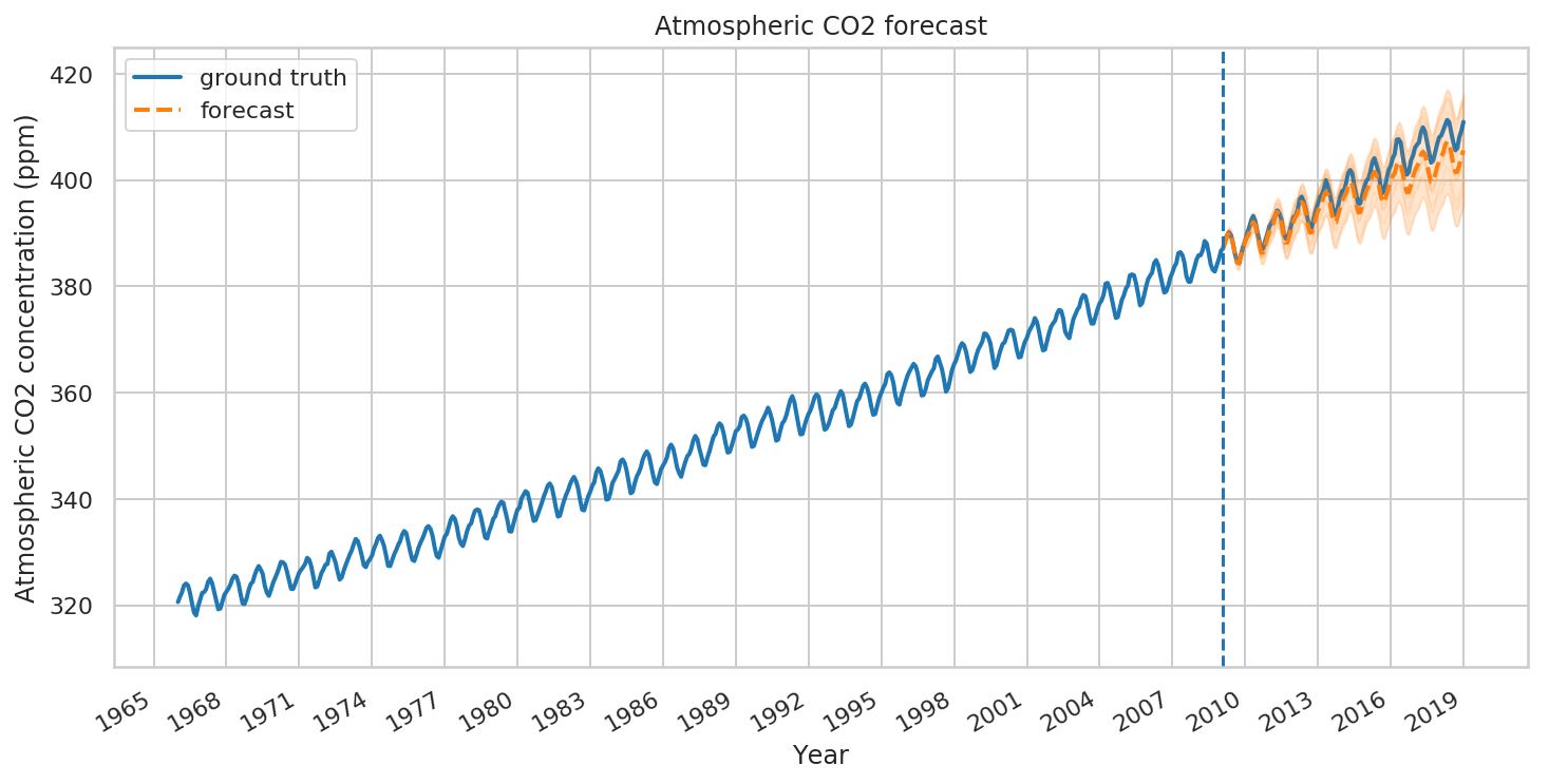
التنبؤ والنقد
الآن دعنا نستخدم النموذج المناسب لبناء توقعات. نحن فقط نسمي tfp.sts.forecast ، والذي يعرض مثيل TensorFlow Distribution الذي يمثل التوزيع التنبئي على الخطوات الزمنية المستقبلية.
co2_forecast_dist = tfp.sts.forecast(
    co2_model,
    observed_time_series=co2_by_month_training_data,
    parameter_samples=q_samples_co2_,
    num_steps_forecast=num_forecast_steps)
على وجه الخصوص ، يمنحنا mean و stddev لتوزيع التوقعات تنبؤًا بعدم اليقين الهامشي في كل خطوة زمنية ، ويمكننا أيضًا استخلاص عينات من العقود الآجلة المحتملة.
num_samples=10

co2_forecast_mean, co2_forecast_scale, co2_forecast_samples = (
    co2_forecast_dist.mean().numpy()[..., 0],
    co2_forecast_dist.stddev().numpy()[..., 0],
    co2_forecast_dist.sample(num_samples).numpy()[..., 0])
fig, ax = plot_forecast(
    co2_dates, co2_by_month,
    co2_forecast_mean, co2_forecast_scale, co2_forecast_samples,
    x_locator=co2_loc,
    x_formatter=co2_fmt,
    title="Atmospheric CO2 forecast")
ax.axvline(co2_dates[-num_forecast_steps], linestyle="--")
ax.legend(loc="upper left")
ax.set_ylabel("Atmospheric CO2 concentration (ppm)")
ax.set_xlabel("Year")
fig.autofmt_xdate()
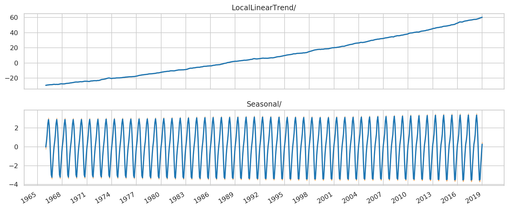
يمكننا أن نفهم أيضًا ملاءمة النموذج من خلال تحليله إلى مساهمات سلاسل زمنية فردية:
# Build a dict mapping components to distributions over
# their contribution to the observed signal.
component_dists = sts.decompose_by_component(
    co2_model,
    observed_time_series=co2_by_month,
    parameter_samples=q_samples_co2_)
co2_component_means_, co2_component_stddevs_ = (
    {k.name: c.mean() for k, c in component_dists.items()},
    {k.name: c.stddev() for k, c in component_dists.items()})
_ = plot_components(co2_dates, co2_component_means_, co2_component_stddevs_,
                    x_locator=co2_loc, x_formatter=co2_fmt)
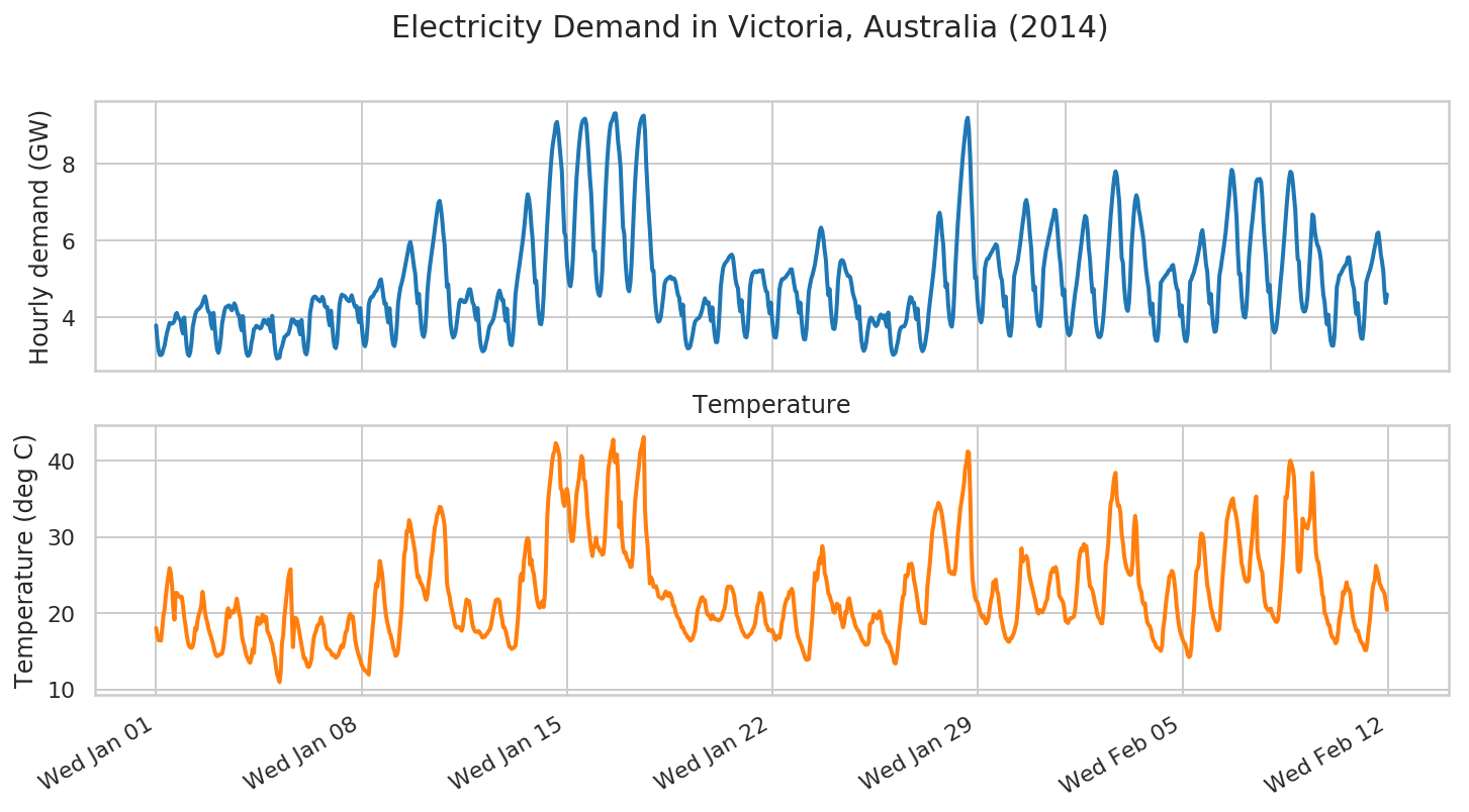
التنبؤ بالطلب على الكهرباء
لننظر الآن في مثال أكثر تعقيدًا: التنبؤ بالطلب على الكهرباء في فيكتوريا أستراليا.
أولاً ، سننشئ مجموعة البيانات:
# Victoria electricity demand dataset, as presented at
# https://otexts.com/fpp2/scatterplots.html
# and downloaded from https://github.com/robjhyndman/fpp2-package/blob/master/data/elecdaily.rda
# This series contains the first eight weeks (starting Jan 1). The original
# dataset was half-hourly data; here we've downsampled to hourly data by taking
# every other timestep.
demand_dates = np.arange('2014-01-01', '2014-02-26', dtype='datetime64[h]')
demand_loc = mdates.WeekdayLocator(byweekday=mdates.WE)
demand_fmt = mdates.DateFormatter('%a %b %d')

demand = np.array("3.794,3.418,3.152,3.026,3.022,3.055,3.180,3.276,3.467,3.620,3.730,3.858,3.851,3.839,3.861,3.912,4.082,4.118,4.011,3.965,3.932,3.693,3.585,4.001,3.623,3.249,3.047,3.004,3.104,3.361,3.749,3.910,4.075,4.165,4.202,4.225,4.265,4.301,4.381,4.484,4.552,4.440,4.233,4.145,4.116,3.831,3.712,4.121,3.764,3.394,3.159,3.081,3.216,3.468,3.838,4.012,4.183,4.269,4.280,4.310,4.315,4.233,4.188,4.263,4.370,4.308,4.182,4.075,4.057,3.791,3.667,4.036,3.636,3.283,3.073,3.003,3.023,3.113,3.335,3.484,3.697,3.723,3.786,3.763,3.748,3.714,3.737,3.828,3.937,3.929,3.877,3.829,3.950,3.756,3.638,4.045,3.682,3.283,3.036,2.933,2.956,2.959,3.157,3.236,3.370,3.493,3.516,3.555,3.570,3.656,3.792,3.950,3.953,3.926,3.849,3.813,3.891,3.683,3.562,3.936,3.602,3.271,3.085,3.041,3.201,3.570,4.123,4.307,4.481,4.533,4.545,4.524,4.470,4.457,4.418,4.453,4.539,4.473,4.301,4.260,4.276,3.958,3.796,4.180,3.843,3.465,3.246,3.203,3.360,3.808,4.328,4.509,4.598,4.562,4.566,4.532,4.477,4.442,4.424,4.486,4.579,4.466,4.338,4.270,4.296,4.034,3.877,4.246,3.883,3.520,3.306,3.252,3.387,3.784,4.335,4.465,4.529,4.536,4.589,4.660,4.691,4.747,4.819,4.950,4.994,4.798,4.540,4.352,4.370,4.047,3.870,4.245,3.848,3.509,3.302,3.258,3.419,3.809,4.363,4.605,4.793,4.908,5.040,5.204,5.358,5.538,5.708,5.888,5.966,5.817,5.571,5.321,5.141,4.686,4.367,4.618,4.158,3.771,3.555,3.497,3.646,4.053,4.687,5.052,5.342,5.586,5.808,6.038,6.296,6.548,6.787,6.982,7.035,6.855,6.561,6.181,5.899,5.304,4.795,4.862,4.264,3.820,3.588,3.481,3.514,3.632,3.857,4.116,4.375,4.462,4.460,4.422,4.398,4.407,4.480,4.621,4.732,4.735,4.572,4.385,4.323,4.069,3.940,4.247,3.821,3.416,3.220,3.124,3.132,3.181,3.337,3.469,3.668,3.788,3.834,3.894,3.964,4.109,4.275,4.472,4.623,4.703,4.594,4.447,4.459,4.137,3.913,4.231,3.833,3.475,3.302,3.279,3.519,3.975,4.600,4.864,5.104,5.308,5.542,5.759,6.005,6.285,6.617,6.993,7.207,7.095,6.839,6.387,6.048,5.433,4.904,4.959,4.425,4.053,3.843,3.823,4.017,4.521,5.229,5.802,6.449,6.975,7.506,7.973,8.359,8.596,8.794,9.030,9.090,8.885,8.525,8.147,7.797,6.938,6.215,6.123,5.495,5.140,4.896,4.812,5.024,5.536,6.293,7.000,7.633,8.030,8.459,8.768,9.000,9.113,9.155,9.173,9.039,8.606,8.095,7.617,7.208,6.448,5.740,5.718,5.106,4.763,4.610,4.566,4.737,5.204,5.988,6.698,7.438,8.040,8.484,8.837,9.052,9.114,9.214,9.307,9.313,9.006,8.556,8.275,7.911,7.077,6.348,6.175,5.455,5.041,4.759,4.683,4.908,5.411,6.199,6.923,7.593,8.090,8.497,8.843,9.058,9.159,9.231,9.253,8.852,7.994,7.388,6.735,6.264,5.690,5.227,5.220,4.593,4.213,3.984,3.891,3.919,4.031,4.287,4.558,4.872,4.963,5.004,5.017,5.057,5.064,5.000,5.023,5.007,4.923,4.740,4.586,4.517,4.236,4.055,4.337,3.848,3.473,3.273,3.198,3.204,3.252,3.404,3.560,3.767,3.896,3.934,3.972,3.985,4.032,4.122,4.239,4.389,4.499,4.406,4.356,4.396,4.106,3.914,4.265,3.862,3.546,3.360,3.359,3.649,4.180,4.813,5.086,5.301,5.384,5.434,5.470,5.529,5.582,5.618,5.636,5.561,5.291,5.000,4.840,4.767,4.364,4.160,4.452,4.011,3.673,3.503,3.483,3.695,4.213,4.810,5.028,5.149,5.182,5.208,5.179,5.190,5.220,5.202,5.216,5.232,5.019,4.828,4.686,4.657,4.304,4.106,4.389,3.955,3.643,3.489,3.479,3.695,4.187,4.732,4.898,4.997,5.001,5.022,5.052,5.094,5.143,5.178,5.250,5.255,5.075,4.867,4.691,4.665,4.352,4.121,4.391,3.966,3.615,3.437,3.430,3.666,4.149,4.674,4.851,5.011,5.105,5.242,5.378,5.576,5.790,6.030,6.254,6.340,6.253,6.039,5.736,5.490,4.936,4.580,4.742,4.230,3.895,3.712,3.700,3.906,4.364,4.962,5.261,5.463,5.495,5.477,5.394,5.250,5.159,5.081,5.083,5.038,4.857,4.643,4.526,4.428,4.141,3.975,4.290,3.809,3.423,3.217,3.132,3.192,3.343,3.606,3.803,3.963,3.998,3.962,3.894,3.814,3.776,3.808,3.914,4.033,4.079,4.027,3.974,4.057,3.859,3.759,4.132,3.716,3.325,3.111,3.030,3.046,3.096,3.254,3.390,3.606,3.718,3.755,3.768,3.768,3.834,3.957,4.199,4.393,4.532,4.516,4.380,4.390,4.142,3.954,4.233,3.795,3.425,3.209,3.124,3.177,3.288,3.498,3.715,4.092,4.383,4.644,4.909,5.184,5.518,5.889,6.288,6.643,6.729,6.567,6.179,5.903,5.278,4.788,4.885,4.363,4.011,3.823,3.762,3.998,4.598,5.349,5.898,6.487,6.941,7.381,7.796,8.185,8.522,8.825,9.103,9.198,8.889,8.174,7.214,6.481,5.611,5.026,5.052,4.484,4.148,3.955,3.873,4.060,4.626,5.272,5.441,5.535,5.534,5.610,5.671,5.724,5.793,5.838,5.908,5.868,5.574,5.276,5.065,4.976,4.554,4.282,4.547,4.053,3.720,3.536,3.524,3.792,4.420,5.075,5.208,5.344,5.482,5.701,5.936,6.210,6.462,6.683,6.979,7.059,6.893,6.535,6.121,5.797,5.152,4.705,4.805,4.272,3.975,3.805,3.775,3.996,4.535,5.275,5.509,5.730,5.870,6.034,6.175,6.340,6.500,6.603,6.804,6.787,6.460,6.043,5.627,5.367,4.866,4.575,4.728,4.157,3.795,3.607,3.537,3.596,3.803,4.125,4.398,4.660,4.853,5.115,5.412,5.669,5.930,6.216,6.466,6.641,6.605,6.316,5.821,5.520,5.016,4.657,4.746,4.197,3.823,3.613,3.505,3.488,3.532,3.716,4.011,4.421,4.836,5.296,5.766,6.233,6.646,7.011,7.380,7.660,7.804,7.691,7.364,7.019,6.260,5.545,5.437,4.806,4.457,4.235,4.172,4.396,5.002,5.817,6.266,6.732,7.049,7.184,7.085,6.798,6.632,6.408,6.218,5.968,5.544,5.217,4.964,4.758,4.328,4.074,4.367,3.883,3.536,3.404,3.396,3.624,4.271,4.916,4.953,5.016,5.048,5.106,5.124,5.200,5.244,5.242,5.341,5.368,5.166,4.910,4.762,4.700,4.276,4.035,4.318,3.858,3.550,3.399,3.382,3.590,4.261,4.937,4.994,5.094,5.168,5.303,5.410,5.571,5.740,5.900,6.177,6.274,6.039,5.700,5.389,5.192,4.672,4.359,4.614,4.118,3.805,3.627,3.646,3.882,4.470,5.106,5.274,5.507,5.711,5.950,6.200,6.527,6.884,7.196,7.615,7.845,7.759,7.437,7.059,6.584,5.742,5.125,5.139,4.564,4.218,4.025,4.000,4.245,4.783,5.504,5.920,6.271,6.549,6.894,7.231,7.535,7.597,7.562,7.609,7.534,7.118,6.448,5.963,5.565,5.005,4.666,4.850,4.302,3.905,3.678,3.610,3.672,3.869,4.204,4.541,4.944,5.265,5.651,6.090,6.547,6.935,7.318,7.625,7.793,7.760,7.510,7.145,6.805,6.103,5.520,5.462,4.824,4.444,4.237,4.157,4.164,4.275,4.545,5.033,5.594,6.176,6.681,6.628,6.238,6.039,5.897,5.832,5.701,5.483,4.949,4.589,4.407,4.027,3.820,4.075,3.650,3.388,3.271,3.268,3.498,4.086,4.800,4.933,5.102,5.126,5.194,5.260,5.319,5.364,5.419,5.559,5.568,5.332,5.027,4.864,4.738,4.303,4.093,4.379,3.952,3.632,3.461,3.446,3.732,4.294,4.911,5.021,5.138,5.223,5.348,5.479,5.661,5.832,5.966,6.178,6.212,5.949,5.640,5.449,5.213,4.678,4.376,4.601,4.147,3.815,3.610,3.605,3.879,4.468,5.090,5.226,5.406,5.561,5.740,5.899,6.095,6.272,6.402,6.610,6.585,6.265,5.925,5.747,5.497,4.932,4.580,4.763,4.298,4.026,3.871,3.827,4.065,4.643,5.317,5.494,5.685,5.814,5.912,5.999,6.097,6.176,6.136,6.131,6.049,5.796,5.532,5.475,5.254,4.742,4.453,4.660,4.176,3.895,3.726,3.717,3.910,4.479,5.135,5.306,5.520,5.672,5.737,5.785,5.829,5.893,5.892,5.921,5.817,5.557,5.304,5.234,5.074,4.656,4.396,4.599,4.064,3.749,3.560,3.475,3.552,3.783,4.045,4.258,4.539,4.762,4.938,5.049,5.037,5.066,5.151,5.197,5.201,5.132,4.908,4.725,4.568,4.222,3.939,4.215,3.741,3.380,3.174,3.076,3.071,3.172,3.328,3.427,3.603,3.738,3.765,3.777,3.705,3.690,3.742,3.859,4.032,4.113,4.032,4.066,4.011,3.712,3.530,3.905,3.556,3.283,3.136,3.146,3.400,4.009,4.717,4.827,4.909,4.973,5.036,5.079,5.160,5.228,5.241,5.343,5.350,5.184,4.941,4.797,4.615,4.160,3.904,4.213,3.810,3.528,3.369,3.381,3.609,4.178,4.861,4.918,5.006,5.102,5.239,5.385,5.528,5.724,5.845,6.048,6.097,5.838,5.507,5.267,5.003,4.462,4.184,4.431,3.969,3.660,3.480,3.470,3.693,4.313,4.955,5.083,5.251,5.268,5.293,5.285,5.308,5.349,5.322,5.328,5.151,4.975,4.741,4.678,4.458,4.056,3.868,4.226,3.799,3.428,3.253,3.228,3.452,4.040,4.726,4.709,4.721,4.741,4.846,4.864,4.868,4.836,4.799,4.890,4.946,4.800,4.646,4.693,4.546,4.117,3.897,4.259,3.893,3.505,3.341,3.334,3.623,4.240,4.925,4.986,5.028,4.987,4.984,4.975,4.912,4.833,4.686,4.710,4.718,4.577,4.454,4.532,4.407,4.064,3.883,4.221,3.792,3.445,3.261,3.221,3.295,3.521,3.804,4.038,4.200,4.226,4.198,4.182,4.078,4.018,4.002,4.066,4.158,4.154,4.084,4.104,4.001,3.773,3.700,4.078,3.702,3.349,3.143,3.052,3.070,3.181,3.327,3.440,3.616,3.678,3.694,3.710,3.706,3.764,3.852,4.009,4.202,4.323,4.249,4.275,4.162,3.848,3.706,4.060,3.703,3.401,3.251,3.239,3.455,4.041,4.743,4.815,4.916,4.931,4.966,5.063,5.218,5.381,5.458,5.550,5.566,5.376,5.104,5.022,4.793,4.335,4.108,4.410,4.008,3.666,3.497,3.464,3.698,4.333,4.998,5.094,5.272,5.459,5.648,5.853,6.062,6.258,6.236,6.226,5.957,5.455,5.066,4.968,4.742,4.304,4.105,4.410".split(",")).astype(np.float32)
temperature = np.array("18.050,17.200,16.450,16.650,16.400,17.950,19.700,20.600,22.350,23.700,24.800,25.900,25.300,23.650,20.700,19.150,22.650,22.650,22.400,22.150,22.050,22.150,21.000,19.500,18.450,17.250,16.300,15.700,15.500,15.450,15.650,16.500,18.100,17.800,19.100,19.850,20.300,21.050,22.800,21.650,20.150,19.300,18.750,17.900,17.350,16.850,16.350,15.700,14.950,14.500,14.350,14.450,14.600,14.600,14.700,15.450,16.700,18.300,20.100,20.650,19.450,20.200,20.250,20.050,20.250,20.950,21.900,21.000,19.900,19.250,17.300,16.300,15.800,15.000,14.400,14.050,13.650,13.500,14.150,15.300,14.800,17.050,18.350,19.450,18.550,18.650,18.850,19.800,19.650,18.900,19.500,17.700,17.350,16.950,16.400,15.950,14.900,14.250,13.050,12.000,11.500,10.950,12.300,16.100,17.100,19.600,21.100,22.600,24.350,25.250,25.750,20.350,15.550,18.300,19.400,19.250,18.550,17.700,16.750,15.800,14.900,14.050,14.100,13.500,13.000,12.950,13.300,13.900,15.400,16.750,17.300,17.750,18.400,18.500,18.800,19.450,18.750,18.400,16.950,15.800,15.350,15.250,15.150,14.900,14.500,14.600,14.400,14.150,14.300,14.500,14.950,15.550,15.800,15.550,16.450,17.500,17.700,18.750,19.600,19.900,19.350,19.550,17.900,16.400,15.550,14.900,14.400,13.950,13.300,12.950,12.650,12.450,12.350,12.150,11.950,14.150,15.850,17.750,19.450,22.150,23.850,23.450,24.950,26.850,26.100,25.150,23.250,21.300,19.850,18.900,18.250,17.450,17.100,16.400,15.550,15.050,14.400,14.550,15.150,17.050,18.850,20.850,24.250,27.700,28.400,30.750,30.700,32.200,31.750,30.650,29.750,28.850,27.850,25.950,24.700,24.850,24.050,23.850,23.500,22.950,22.200,21.750,22.350,24.050,25.150,27.100,28.050,29.750,31.250,31.900,32.950,33.150,33.950,33.850,33.250,32.500,31.500,28.300,23.900,22.900,22.300,21.250,20.500,19.850,18.850,18.300,18.100,18.200,18.150,18.000,17.700,18.250,19.700,20.750,21.800,21.500,21.600,20.800,19.400,18.400,17.900,17.600,17.550,17.550,17.650,17.400,17.150,16.800,17.000,16.900,17.200,17.350,17.650,17.800,18.400,19.300,20.200,21.050,21.700,21.800,21.800,21.500,20.000,19.300,18.200,18.100,17.700,16.950,16.250,15.600,15.500,15.300,15.450,15.500,15.750,17.350,19.150,21.650,24.700,25.200,24.300,26.900,28.100,29.450,29.850,29.450,26.350,27.050,25.700,25.150,23.850,22.450,21.450,20.850,20.700,21.300,21.550,20.800,22.300,26.300,32.600,35.150,36.800,38.150,39.950,40.850,41.250,42.300,41.950,41.350,40.600,36.350,36.150,34.600,34.050,35.400,36.300,35.550,33.700,30.650,29.450,29.500,31.000,33.300,35.700,36.650,37.650,39.400,40.600,40.250,37.550,37.300,35.400,32.750,31.200,29.600,28.350,27.500,28.750,28.900,29.900,28.700,28.650,28.150,28.250,27.650,27.800,29.450,32.500,35.750,38.850,39.900,41.100,41.800,42.750,39.900,39.750,40.800,37.950,31.250,34.600,30.250,28.500,27.900,27.950,27.300,26.900,26.800,26.050,26.100,27.700,31.850,34.850,36.350,38.000,39.200,41.050,41.600,42.350,43.100,33.500,30.700,29.100,26.400,23.900,24.700,24.350,23.450,23.450,23.550,23.050,22.200,22.100,22.000,21.900,22.050,22.550,22.850,22.450,22.250,22.650,22.350,21.900,21.000,20.950,20.200,19.700,19.400,19.200,18.650,18.150,18.150,17.650,17.350,17.150,16.800,16.750,16.400,16.500,16.700,17.300,17.750,19.200,20.400,20.900,21.450,22.000,22.100,21.600,21.700,20.500,19.850,19.750,19.500,19.200,19.800,19.500,19.200,19.200,19.150,19.050,19.100,19.250,19.550,20.200,20.550,21.450,23.150,23.500,23.400,23.500,23.300,22.850,22.250,20.950,19.750,19.450,18.900,18.450,17.950,17.550,17.300,16.950,16.900,16.850,17.100,17.250,17.400,17.850,18.100,18.600,19.700,21.000,21.400,22.650,22.550,22.000,21.050,19.550,18.550,18.300,17.750,17.800,17.650,17.800,17.450,16.950,16.500,16.900,17.050,16.750,17.300,18.800,19.350,20.750,21.400,21.900,21.950,22.800,22.750,23.200,22.650,20.800,19.250,17.800,16.950,16.550,16.050,15.750,15.150,14.700,14.150,13.900,13.900,14.000,15.800,17.650,19.700,22.500,25.300,24.300,24.650,26.450,27.250,26.550,28.800,27.850,25.200,24.750,23.750,22.550,22.350,21.700,21.300,20.300,20.050,20.500,21.250,20.850,21.000,19.400,18.900,18.150,18.650,20.200,20.000,21.650,21.950,21.150,20.400,19.500,19.150,18.400,18.050,17.750,17.600,17.150,16.750,16.350,16.250,15.900,15.850,15.900,16.200,18.500,18.750,18.800,19.850,19.750,19.600,19.300,20.000,20.250,19.700,18.600,17.400,17.100,16.650,16.250,16.250,15.800,15.350,14.800,14.250,13.500,13.400,14.350,15.800,17.700,19.000,21.050,22.200,22.450,24.950,24.750,25.050,26.400,26.200,26.500,25.850,24.400,23.600,22.650,21.500,20.150,19.900,18.850,18.700,18.750,18.650,20.050,23.450,24.900,26.450,28.550,30.600,31.550,32.800,33.500,33.700,34.450,34.200,33.650,32.900,31.750,30.500,29.250,28.100,26.450,25.400,25.400,25.150,25.400,25.100,25.950,28.100,30.400,32.000,33.750,34.700,35.800,37.000,39.050,39.750,41.200,41.050,36.050,28.250,24.450,23.150,22.050,21.600,21.450,20.800,20.250,19.700,19.400,19.650,19.100,18.650,18.900,19.400,20.700,21.750,22.350,24.100,23.350,24.400,22.950,22.400,20.950,19.600,18.900,18.000,17.400,16.800,16.550,16.300,16.250,16.750,16.700,17.100,17.500,18.150,18.850,20.650,22.600,25.600,28.500,26.750,27.200,27.300,27.500,27.000,25.450,24.500,23.850,23.200,22.550,21.850,21.050,20.200,19.950,20.400,20.300,20.100,20.450,20.900,21.450,21.800,23.250,24.100,25.200,25.550,25.900,25.450,26.050,25.350,23.900,22.250,22.000,21.700,21.450,20.550,19.000,18.850,18.700,19.050,19.350,19.350,19.450,19.600,20.550,22.400,24.550,26.900,27.950,28.500,28.200,29.050,28.700,28.800,27.150,24.900,23.500,23.350,23.000,22.300,21.400,20.700,19.850,19.400,19.250,18.700,18.650,20.200,23.400,26.400,27.450,29.150,32.050,34.500,34.950,36.550,37.850,38.400,35.150,34.050,34.100,33.100,30.300,29.300,27.550,26.600,25.900,25.500,25.150,25.000,25.150,27.000,31.150,32.750,31.500,26.900,23.900,23.150,22.850,21.500,21.150,21.300,19.700,18.800,18.450,18.300,17.800,16.850,16.400,16.150,15.700,15.500,15.400,15.300,15.050,15.650,18.100,19.200,21.050,22.350,23.450,24.850,24.950,25.550,25.300,24.250,22.750,20.850,19.350,18.250,17.450,17.000,16.500,16.100,15.950,15.300,14.550,14.250,14.400,15.550,18.300,20.000,22.750,25.450,25.800,26.350,29.150,30.450,30.350,29.600,27.550,25.550,23.650,22.950,21.850,20.700,20.150,19.300,19.000,18.400,17.800,17.750,18.000,20.800,23.400,25.750,27.750,29.600,32.150,32.900,33.650,34.300,34.800,35.050,33.750,33.250,32.400,31.250,29.650,28.550,26.550,25.950,25.000,24.400,24.150,24.150,24.350,26.900,28.750,30.350,32.750,34.250,35.300,28.400,27.250,26.600,25.750,25.350,23.150,21.550,20.850,20.550,20.350,20.550,20.600,19.900,19.550,19.200,18.900,18.850,19.250,21.000,23.050,25.350,27.700,31.050,35.250,35.100,36.850,39.250,40.000,39.450,38.950,37.750,33.850,30.400,25.700,25.400,25.600,28.150,32.400,31.850,31.350,31.200,31.100,31.950,32.450,35.200,38.400,35.850,30.700,27.850,26.900,26.650,25.250,24.450,22.500,22.050,20.000,19.750,19.100,18.500,18.400,17.400,16.900,16.800,16.450,16.050,16.300,17.450,19.300,20.000,21.050,22.800,22.550,23.300,24.050,23.100,23.100,22.500,20.800,19.550,18.800,18.200,17.650,17.750,17.150,16.550,16.200,16.000,15.600,15.150,15.150,16.250,17.800,19.150,21.000,22.800,23.850,24.250,26.200,25.650,25.050,23.850,23.600,23.100,22.950,22.550,21.550,20.450,19.600,18.700,18.300,18.000,17.550,17.300,17.200,17.950,19.450,21.100,23.050,24.650,25.050,25.850,25.300,26.650,25.500,25.900,26.250,25.300,25.150,23.600,22.050,21.700,21.150,20.550,20.500,20.200,20.500,20.600,20.900,21.700,22.000,22.250,23.400,23.900,25.250,26.200,26.000,25.300,25.200,25.300,25.500,25.350,25.050,24.850,24.050,23.150,22.300,21.900,21.150,20.300,19.650,19.700,19.750,20.250,21.500,23.600,24.600,25.900,25.450,24.850,25.900,26.150,26.250,26.350,26.250,25.850,25.300,24.600,23.750,22.250,21.750,21.450,21.500,21.300,21.250,21.200,21.600,22.000,23.650,25.200,26.400,25.500,25.150,26.950,28.350,25.650,25.000,25.500,24.150,22.900,21.600,21.750,21.500,21.550,20.450,19.500,18.750,18.650,18.200,17.300,17.900,18.050,17.400,16.850,17.950,20.550,21.950,22.600,22.300,22.400,22.300,21.100,20.250,19.200,18.900,18.600,18.350,17.700,17.200,16.850,16.900,16.800,16.800,16.600,16.350,17.200,18.350,19.550,20.300,21.600,21.800,23.300,23.200,24.550,24.950,24.900,23.700,22.000,19.650,18.250,17.700,17.250,16.900,16.550,16.050,16.450,15.400,14.900,14.700,16.100,18.450,19.800,23.000,25.250,27.600,27.900,28.550,29.450,29.700,29.350,27.000,23.550,21.900,20.750,20.150,19.600,19.150,18.800,18.550,18.200,17.750,17.650,17.800,18.750,19.600,20.450,21.950,23.700,23.150,24.150,24.550,21.400,19.150,19.050,16.500,15.900,14.850,15.300,14.100,13.800,13.600,13.450,13.400,13.050,12.750,12.800,12.750,13.600,14.950,16.100,17.500,18.500,19.300,19.400,19.750,19.400,19.450,19.450,18.900,17.650,16.800,15.900,15.050,14.550,14.250,13.800,13.850,13.700,13.650,13.350,13.400,14.050,15.000,16.650,17.850,18.450,18.200,18.900,19.850,20.000,19.700,18.800,17.500,16.600,16.250,16.000,16.300,16.400,15.800,15.850,14.600,14.650,15.200,14.900,14.600,15.150,16.000,16.350,17.000,18.300,19.050,19.300,19.400,18.650,18.750,19.100,18.300,17.950,17.550,16.900,16.450,15.850,15.800,15.650,15.200,14.700,14.950,15.250,15.200,15.800,16.800,17.900,19.700,21.050,21.600,22.550,22.750,22.900,22.500,21.950,20.450,19.600,19.200,18.000,16.950,16.450,16.150,15.600,15.150,15.250,15.200,14.750,15.050,15.600,17.750,18.450,20.050,21.350,22.500,23.550,24.100,22.600,23.150,24.100,22.650,21.250,19.900,19.100,18.250,17.750,17.500,16.600,16.100,15.850,15.750,15.700,16.350,19.600,25.750,27.800,30.050,32.350,31.900,32.450,29.600,28.850,23.450,21.100,20.100,20.100,19.900,19.300,19.050,18.850".split(",")).astype(np.float32)

num_forecast_steps = 24 * 7 * 2 # Two weeks.
demand_training_data = demand[:-num_forecast_steps]
colors = sns.color_palette()
c1, c2 = colors[0], colors[1]

fig = plt.figure(figsize=(12, 6))
ax = fig.add_subplot(2, 1, 1)
ax.plot(demand_dates[:-num_forecast_steps],
        demand[:-num_forecast_steps], lw=2, label="training data")
ax.set_ylabel("Hourly demand (GW)")

ax = fig.add_subplot(2, 1, 2)

ax.plot(demand_dates[:-num_forecast_steps],
        temperature[:-num_forecast_steps], lw=2, label="training data", c=c2)
ax.set_ylabel("Temperature (deg C)")
ax.set_title("Temperature")
ax.xaxis.set_major_locator(demand_loc)
ax.xaxis.set_major_formatter(demand_fmt)
fig.suptitle("Electricity Demand in Victoria, Australia (2014)",
             fontsize=15)
fig.autofmt_xdate()
النموذج والتركيب
يجمع نموذجنا بين موسمية الساعة من اليوم ويوم الأسبوع ، مع نموذج الانحدار الخطي لتأثير درجة الحرارة ، وعملية الانحدار الذاتي للتعامل مع بقايا التباين المحدود.
def build_model(observed_time_series):
  hour_of_day_effect = sts.Seasonal(
      num_seasons=24,
      observed_time_series=observed_time_series,
      name='hour_of_day_effect')
  day_of_week_effect = sts.Seasonal(
      num_seasons=7, num_steps_per_season=24,
      observed_time_series=observed_time_series,
      name='day_of_week_effect')
  temperature_effect = sts.LinearRegression(
      design_matrix=tf.reshape(temperature - np.mean(temperature),
                               (-1, 1)), name='temperature_effect')
  autoregressive = sts.Autoregressive(
      order=1,
      observed_time_series=observed_time_series,
      name='autoregressive')
  model = sts.Sum([hour_of_day_effect,
                   day_of_week_effect,
                   temperature_effect,
                   autoregressive],
                   observed_time_series=observed_time_series)
  return model
كما هو مذكور أعلاه ، سنقوم بتلائم النموذج مع الاستدلال المتغير وسحب عينات من النموذج الخلفي.
demand_model = build_model(demand_training_data)

# Build the variational surrogate posteriors `qs`.
variational_posteriors = tfp.sts.build_factored_surrogate_posterior(
    model=demand_model)
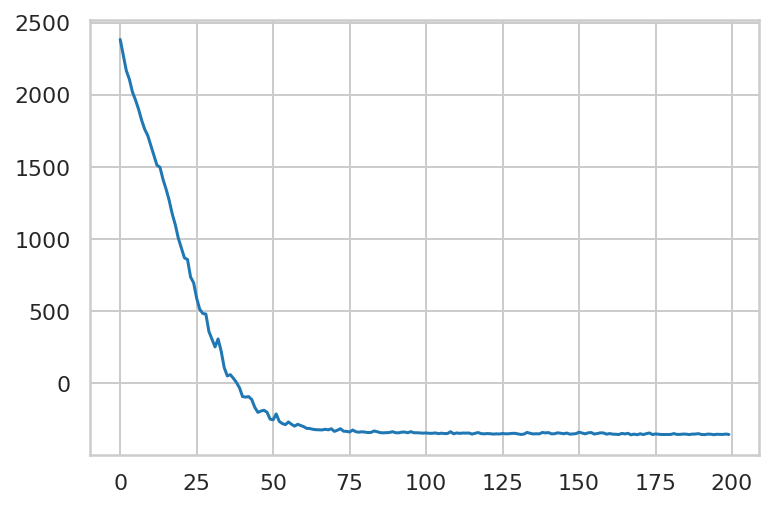
تقليل الخسارة المتغيرة.
# Allow external control of optimization to reduce test runtimes.
num_variational_steps = 200 # @param { isTemplate: true}
num_variational_steps = int(num_variational_steps)

# Build and optimize the variational loss function.
elbo_loss_curve = tfp.vi.fit_surrogate_posterior(
    target_log_prob_fn=demand_model.joint_distribution(
        observed_time_series=demand_training_data).log_prob,
    surrogate_posterior=variational_posteriors,
    optimizer=tf.optimizers.Adam(learning_rate=0.1),
    num_steps=num_variational_steps,
    jit_compile=True)
plt.plot(elbo_loss_curve)
plt.show()

# Draw samples from the variational posterior.
q_samples_demand_ = variational_posteriors.sample(50)
print("Inferred parameters:")
for param in demand_model.parameters:
  print("{}: {} +- {}".format(param.name,
                              np.mean(q_samples_demand_[param.name], axis=0),
                              np.std(q_samples_demand_[param.name], axis=0)))
Inferred parameters:
observation_noise_scale: 0.010157477110624313 +- 0.0026443174574524164
hour_of_day_effect/_drift_scale: 0.0019522204529494047 +- 0.0011986979516223073
day_of_week_effect/_drift_scale: 0.013334915973246098 +- 0.01825258508324623
temperature_effect/_weights: [0.06648794] +- [0.00411669]
autoregressive/_coefficients: [0.9871232] +- [0.00413899]
autoregressive/_level_scale: 0.14199139177799225 +- 0.002658574376255274
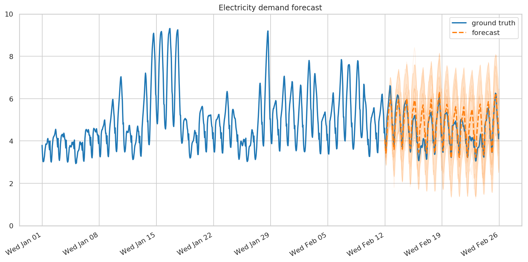
التنبؤ والنقد
مرة أخرى ، نقوم بإنشاء توقع ببساطة عن طريق استدعاء tfp.sts.forecast مع نموذجنا ، وسلسلة الوقت ، والمعلمات التي تم أخذ عينات منها.
demand_forecast_dist = tfp.sts.forecast(
    model=demand_model,
    observed_time_series=demand_training_data,
    parameter_samples=q_samples_demand_,
    num_steps_forecast=num_forecast_steps)
num_samples=10

(
    demand_forecast_mean,
    demand_forecast_scale,
    demand_forecast_samples
) = (
    demand_forecast_dist.mean().numpy()[..., 0],
    demand_forecast_dist.stddev().numpy()[..., 0],
    demand_forecast_dist.sample(num_samples).numpy()[..., 0]
    )
fig, ax = plot_forecast(demand_dates, demand,
                        demand_forecast_mean,
                        demand_forecast_scale,
                        demand_forecast_samples,
                        title="Electricity demand forecast",
                        x_locator=demand_loc, x_formatter=demand_fmt)
ax.set_ylim([0, 10])
fig.tight_layout()
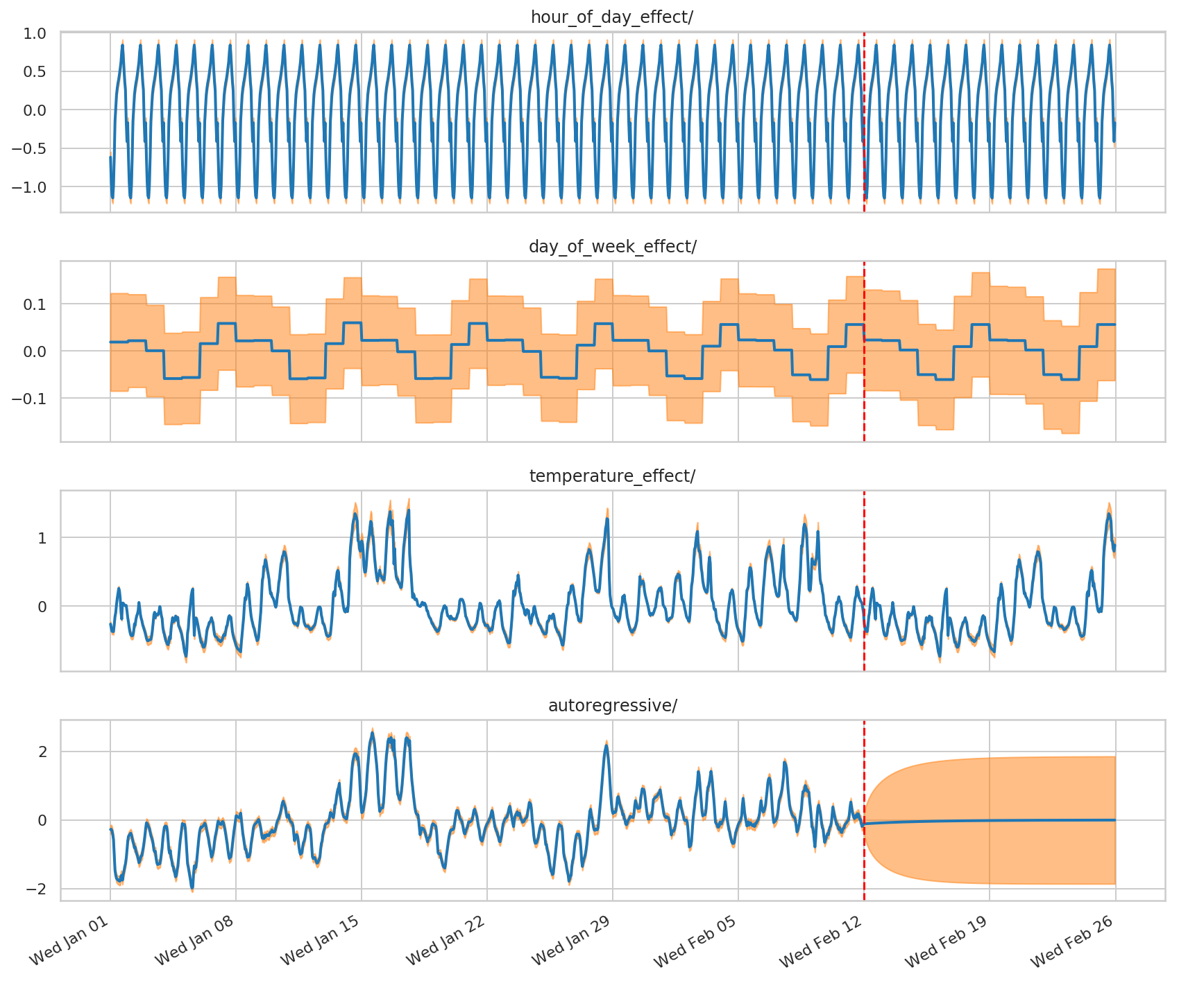
دعنا نتخيل تحلل السلسلة المرصودة والمتوقعة إلى المكونات الفردية:
# Get the distributions over component outputs from the posterior marginals on
# training data, and from the forecast model.
component_dists = sts.decompose_by_component(
    demand_model,
    observed_time_series=demand_training_data,
    parameter_samples=q_samples_demand_)

forecast_component_dists = sts.decompose_forecast_by_component(
    demand_model,
    forecast_dist=demand_forecast_dist,
    parameter_samples=q_samples_demand_)
demand_component_means_, demand_component_stddevs_ = (
    {k.name: c.mean() for k, c in component_dists.items()},
    {k.name: c.stddev() for k, c in component_dists.items()})

(
    demand_forecast_component_means_,
    demand_forecast_component_stddevs_
) = (
    {k.name: c.mean() for k, c in forecast_component_dists.items()},
    {k.name: c.stddev() for k, c in forecast_component_dists.items()}
    )
# Concatenate the training data with forecasts for plotting.
component_with_forecast_means_ = collections.OrderedDict()
component_with_forecast_stddevs_ = collections.OrderedDict()
for k in demand_component_means_.keys():
  component_with_forecast_means_[k] = np.concatenate([
      demand_component_means_[k],
      demand_forecast_component_means_[k]], axis=-1)
  component_with_forecast_stddevs_[k] = np.concatenate([
      demand_component_stddevs_[k],
      demand_forecast_component_stddevs_[k]], axis=-1)


fig, axes = plot_components(
  demand_dates,
  component_with_forecast_means_,
  component_with_forecast_stddevs_,
  x_locator=demand_loc, x_formatter=demand_fmt)
for ax in axes.values():
  ax.axvline(demand_dates[-num_forecast_steps], linestyle="--", color='red')
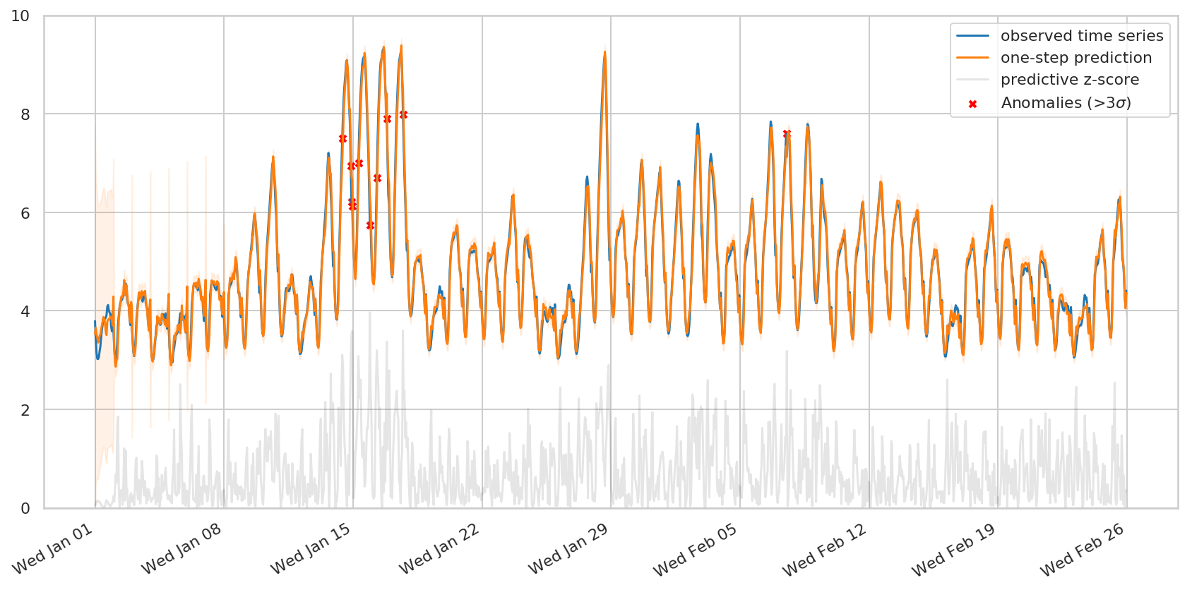
إذا أردنا اكتشاف الحالات الشاذة في السلسلة المرصودة ، فقد نكون مهتمين أيضًا بالتوزيعات التنبؤية ذات الخطوة الواحدة: التنبؤ لكل خطوة زمنية ، مع الأخذ في الاعتبار فقط الخطوات الزمنية حتى تلك النقطة. يحسب tfp.sts.one_step_predictive جميع التوزيعات التنبؤية ذات الخطوة الواحدة في مسار واحد:
demand_one_step_dist = sts.one_step_predictive(
    demand_model,
    observed_time_series=demand,
    parameter_samples=q_samples_demand_)

demand_one_step_mean, demand_one_step_scale = (
    demand_one_step_dist.mean().numpy(), demand_one_step_dist.stddev().numpy())
مخطط بسيط لاكتشاف الشذوذ هو وضع علامة على جميع الخطوات الزمنية حيث تكون الملاحظات أكثر من ثلاثة stddevs من القيمة المتوقعة - هذه هي الخطوات الزمنية الأكثر إثارة للدهشة وفقًا للنموذج.
fig, ax = plot_one_step_predictive(
    demand_dates, demand,
    demand_one_step_mean, demand_one_step_scale,
    x_locator=demand_loc, x_formatter=demand_fmt)
ax.set_ylim(0, 10)

# Use the one-step-ahead forecasts to detect anomalous timesteps.
zscores = np.abs((demand - demand_one_step_mean) /
                 demand_one_step_scale)
anomalies = zscores > 3.0
ax.scatter(demand_dates[anomalies],
           demand[anomalies],
           c="red", marker="x", s=20, linewidth=2, label=r"Anomalies (>3$\sigma$)")
ax.plot(demand_dates, zscores, color="black", alpha=0.1, label='predictive z-score')
ax.legend()
plt.show()