| | |  צפה במקור ב-GitHub צפה במקור ב-GitHub | |
זהו יציאת TensorFlow Probability של המאמר המכונה 16 במרץ 2020 מאת Li et al. אנו משחזרים נאמנה את השיטות והתוצאות של המחברים המקוריים בפלטפורמת TensorFlow Probability, ומציגים כמה מהיכולות של TFP במסגרת מודלים אפידמיולוגיים מודרניים. העברה ל-TensorFlow נותנת לנו מהירות של ~10x ביחס לקוד ה-Matlab המקורי, ומכיוון ש-TensorFlow Probability תומכת באופן נרחב בחישוב אצווה וקטורי, גם משתנה בצורה חיובית למאות שכפולים עצמאיים.
דף מקורי
Ruiyun Li, Sen Pei, Bin Chen, Yimeng Song, Tao Zhang, Wan Yang וג'פרי שאמאן. זיהום לא מתועד מהותי מקל על הפצה מהירה של נגיף קורונה חדש (SARS-CoV2). (2020), דוי: https://doi.org/10.1126/science.abb3221 .
תקציר:. "ההערכה השכיחות ואת מדבקת קורונה רומן מתועד (SARS-CoV2) זיהומים היא קריטית להבנת שכיחות הכוללת פוטנציאל מגיף של מחלה זו הנה אנו משתמשים תצפיות של זיהום לדווח בתוך סין, בשילוב עם נתונים ניידים, מודל מטה-אוכלוסיה דינמי מרושת והסקת בייסיאנית, כדי להסיק מאפיינים אפידמיולוגיים קריטיים הקשורים ל-SARS-CoV2, כולל חלקם של זיהומים לא מתועדים והמידבקות שלהם. אנו מעריכים ש-86% מכלל הזיהומים היו לא מתועדים (95% CI: [82%-90%] ) לפני הגבלות נסיעה ל-23 בינואר 2020. לאדם, שיעור ההעברה של זיהומים לא מתועדים היה 55% מהזיהומים המתועדים ([46%–62%)), אך עם זאת, בשל מספרם הגדול יותר, זיהומים לא מתועדים היו מקור ההדבקה ל-79 % מהמקרים המתועדים. ממצאים אלה מסבירים את ההתפשטות הגיאוגרפית המהירה של SARS-CoV2 ומצביעים על כך שהבלימה של הנגיף הזה תהיה מאתגרת במיוחד."
Github לקשר לקוד ונתונים.
סקירה כללית
המודל הוא מודל המחלה compartmental , ובה מדורים "רגישים", "חשופים" (נגוע אך טרם זיהומיות), "אף פעם לא מתועד זיהומיות", ו "בסופו של דבר מתועד זיהומיות". ישנם שני מאפיינים ראויים לציון: תאים נפרדים לכל אחת מ-375 ערים סיניות, עם הנחה לגבי האופן שבו אנשים נוסעים מעיר אחת לאחרת; ועיכובים בדיווח זיהום, כך במקרה זה הופך "בסופו של דבר מתועד זיהומיות" ביום \(t\) אינו מופיע ברשימת הספירה במקרה שנצפתה עד יום סטוכסטיים מאוחר.
המודל מניח שהמקרים שלא תועדו בסופו של דבר לא מתועדים בהיותם קלים יותר, וכך מדביקים אחרים בשיעור נמוך יותר. הפרמטר העיקרי המעניין במאמר המקורי הוא שיעור המקרים שלא מתועדים, כדי להעריך הן את היקף ההדבקה הקיימת והן את ההשפעה של העברה לא מתועדת על התפשטות המחלה.
קולב זה בנוי כהדרכה בקוד בסגנון מלמטה למעלה. לפי הסדר, נעשה
- להטמיע ולבחון בקצרה את הנתונים,
- הגדר את מרחב המצב והדינמיקה של המודל,
- בנה חבילת פונקציות לביצוע הסקת מסקנות במודל בעקבות Li et al, ו
- פנה אליהם ובחן את התוצאות. ספוילר: הם יוצאים כמו הנייר.
התקנה וייבוא פייתון
pip3 install -q tf-nightly tfp-nightly
import collections
import io
import requests
import time
import zipfile

import matplotlib.pyplot as plt
import numpy as np
import pandas as pd

import tensorflow.compat.v2 as tf
import tensorflow_probability as tfp
from tensorflow_probability.python.internal import samplers

tfd = tfp.distributions
tfes = tfp.experimental.sequential
ייבוא נתונים
בואו לייבא את הנתונים מ-github ונבדוק חלק מהם.
r = requests.get('https://raw.githubusercontent.com/SenPei-CU/COVID-19/master/Data.zip')
z = zipfile.ZipFile(io.BytesIO(r.content))
z.extractall('/tmp/')
raw_incidence = pd.read_csv('/tmp/data/Incidence.csv')
raw_mobility = pd.read_csv('/tmp/data/Mobility.csv')
raw_population = pd.read_csv('/tmp/data/pop.csv')
להלן נוכל לראות את ספירת ההיארעות הגולמית ליום. אנחנו הכי מתעניינים ב-14 הימים הראשונים (10 בינואר עד 23 בינואר), שכן מגבלות הנסיעה הוקמו ב-23. המאמר עוסק בכך באמצעות מודלים של 10-23 בינואר ו-23 בינואר+ בנפרד, עם פרמטרים שונים; רק נגביל את ההעתקה שלנו לתקופה המוקדמת יותר.
raw_incidence.drop('Date', axis=1)  # The 'Date' column is all 1/18/21
# Luckily the days are in order, starting on January 10th, 2020.
בואו נבדוק את ספירת ההיארעות של ווהאן.
plt.plot(raw_incidence.Wuhan, '.-')
plt.title('Wuhan incidence counts over 1/10/20 - 02/08/20')
plt.show()
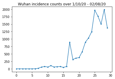
בינתיים הכל טוב. כעת האוכלוסייה הראשונית נחשבת.
raw_population
בואו גם נבדוק ותרשום איזה ערך הוא ווהאן.
raw_population['City'][169]
'Wuhan'
WUHAN_IDX = 169
וכאן אנו רואים את מטריצת הניידות בין ערים שונות. זהו פרוקסי למספר האנשים שעוברים בין ערים שונות ב-14 הימים הראשונים. זה נגזר מרשומות GPS שסיפקה Tencent עבור עונת ראש השנה הירחית 2018. Li et al ניידות מודל בעונת 2020 כפי ידוע כמה (בכפוף היקש) גורם קבוע \(\theta\) פעמים זה.
raw_mobility
לבסוף, בוא נעבד את כל זה מראש למערכים נראים שנוכל לצרוך.
# The given populations are only "initial" because of intercity mobility during
# the holiday season.
initial_population = raw_population['Population'].to_numpy().astype(np.float32)
המר את נתוני הניידות לטנזור בצורת [L, L, T], כאשר L הוא מספר המיקומים, ו-T הוא מספר שלבי הזמן.
daily_mobility_matrices = []
for i in range(1, 15):
  day_mobility = raw_mobility[raw_mobility['Day'] == i]

  # Make a matrix of daily mobilities.
  z = pd.crosstab(
      day_mobility.Origin,
      day_mobility.Destination,
      values=day_mobility['Mobility Index'], aggfunc='sum', dropna=False)

  # Include every city, even if there are no rows for some in the raw data on
  # some day.  This uses the sort order of `raw_population`.
  z = z.reindex(index=raw_population['City'], columns=raw_population['City'],
                fill_value=0)
  # Finally, fill any missing entries with 0. This means no mobility.
  z = z.fillna(0)
  daily_mobility_matrices.append(z.to_numpy())

mobility_matrix_over_time = np.stack(daily_mobility_matrices, axis=-1).astype(
    np.float32)
לבסוף קח את הזיהומים שנצפו וערוך טבלה [L, T].
# Remove the date parameter and take the first 14 days.
observed_daily_infectious_count = raw_incidence.to_numpy()[:14, 1:]
observed_daily_infectious_count = np.transpose(
    observed_daily_infectious_count).astype(np.float32)
ובדקו פעמיים שקיבלנו את הצורות כמו שרצינו. כזכור, אנו עובדים עם 375 ערים ו-14 ימים.
print('Mobility Matrix over time should have shape (375, 375, 14): {}'.format(
    mobility_matrix_over_time.shape))
print('Observed Infectious should have shape (375, 14): {}'.format(
    observed_daily_infectious_count.shape))
print('Initial population should have shape (375): {}'.format(
    initial_population.shape))
Mobility Matrix over time should have shape (375, 375, 14): (375, 375, 14)
Observed Infectious should have shape (375, 14): (375, 14)
Initial population should have shape (375): (375,)
הגדרת מצב ופרמטרים
בואו נתחיל להגדיר את המודל שלנו. המודל שאנחנו משחזרים הינה נגזרת של דגם שעיר . במקרה זה יש לנו את המצבים הבאים משתנים בזמן:
- \(S\): מספר אנשים רגישים המחלה בכל עיר.
- \(E\): מספר אנשים בכל עיר חשופים למחלה אך לא זיהומיות עדיין. מבחינה ביולוגית, זה מתאים להידבקות במחלה, בכך שכל האנשים שנחשפו הופכים בסופו של דבר לזיהומים.
- \(I^u\): מספר אנשים בכל עיר שהם זיהומיות אבל מתועד. במודל זה בעצם אומר "לעולם לא יתועד".
- \(I^r\): מספר אנשים בכל עיר אשר מידבקים, תועדו ככאלה. Li et al עיכובים בדיווח המודל, כך \(I^r\) בעצם מתאים משהו כמו "המקרה הוא חמור מספיק כדי להיות מתועד בשלב כלשהו בעתיד".
כפי שנראה להלן, נסיק את המצבים הללו על ידי הפעלת מסנן קלמן (EAKF) מותאם אנסמבל קדימה בזמן. וקטור המצב של EAKF הוא וקטור אחד עם אינדקס עיר עבור כל אחת מהכמויות הללו.
למודל יש את הפרמטרים הגלובליים הבאים, בלתי משתנים בזמן:
- \(\beta\): תעריף ההולכה בשל יחידים זיהומיות מתועד.
- \(\mu\): תעריף ההולכה יחסית בשל יחידים מתועדים-זיהומיות. זה יפעל באמצעות המוצר \(\mu \beta\).
- \(\theta\): הגורם ניידות בינעירוניים. זהו פקטור גדול מ-1 המתקן עבור תת דיווח של נתוני ניידות (ולגידול האוכלוסייה מ-2018 עד 2020).
- \(Z\): תקופת הדגירה הממוצע (כלומר, הזמן במצב "חשופים").
- \(\alpha\): זהו שבריר של זיהומים חמורים מספיק כדי להיות (בסופו של דבר) מתועד.
- \(D\): משך זיהומים הממוצע (כלומר, זמן בכל אחת משתי המדינות "מדבקת").
אנו נסיק הערכות נקודות עבור פרמטרים אלה עם לולאה איטרטיבית-סינון סביב ה-EAKF עבור המדינות.
המודל תלוי גם בקבועים לא מוסקים:
- \(M\): המטריצה ניידות בינעירוניים. זה משתנה בזמן ונראה שניתן. תזכיר כי זה מדורג על ידי הפרמטר להסיק \(\theta\) לתת תנועות האוכלוסייה בפועל בין הערים.
- \(N\): המספר הכולל של אנשים בכל עיר. האוכלוסיות הראשוניות כנתון, ואת הזמן-הווריאציה של אוכלוסייה מחושבת מן המספרים ניידות \(\theta M\).
ראשית, אנו נותנים לעצמנו כמה מבני נתונים לשמירה על המצבים והפרמטרים שלנו.
SEIRComponents = collections.namedtuple(
  typename='SEIRComponents',
  field_names=[
    'susceptible',              # S
    'exposed',                  # E
    'documented_infectious',    # I^r
    'undocumented_infectious',  # I^u
    # This is the count of new cases in the "documented infectious" compartment.
    # We need this because we will introduce a reporting delay, between a person
    # entering I^r and showing up in the observable case count data.
    # This can't be computed from the cumulative `documented_infectious` count,
    # because some portion of that population will move to the 'recovered'
    # state, which we aren't tracking explicitly.
    'daily_new_documented_infectious'])

ModelParams = collections.namedtuple(
    typename='ModelParams',
    field_names=[
      'documented_infectious_tx_rate',             # Beta
      'undocumented_infectious_tx_relative_rate',  # Mu
      'intercity_underreporting_factor',           # Theta
      'average_latency_period',                    # Z
      'fraction_of_documented_infections',         # Alpha
      'average_infection_duration'                 # D
    ]
)
אנו מקודדים גם את הגבולות של Li et al עבור ערכי הפרמטרים.
PARAMETER_LOWER_BOUNDS = ModelParams(
    documented_infectious_tx_rate=0.8,
    undocumented_infectious_tx_relative_rate=0.2,
    intercity_underreporting_factor=1.,
    average_latency_period=2.,
    fraction_of_documented_infections=0.02,
    average_infection_duration=2.
)

PARAMETER_UPPER_BOUNDS = ModelParams(
    documented_infectious_tx_rate=1.5,
    undocumented_infectious_tx_relative_rate=1.,
    intercity_underreporting_factor=1.75,
    average_latency_period=5.,
    fraction_of_documented_infections=1.,
    average_infection_duration=5.
)
SEIR Dynamics
כאן אנו מגדירים את הקשר בין הפרמטרים למצב.
משוואות הזמן-דינמיקה מ-Li et al (חומר משלים, משוואות 1-5) הן כדלקמן:
\(\frac{dS_i}{dt} = -\beta \frac{S_i I_i^r}{N_i} - \mu \beta \frac{S_i I_i^u}{N_i} + \theta \sum_k \frac{M_{ij} S_j}{N_j - I_j^r} - + \theta \sum_k \frac{M_{ji} S_j}{N_i - I_i^r}\)
\(\frac{dE_i}{dt} = \beta \frac{S_i I_i^r}{N_i} + \mu \beta \frac{S_i I_i^u}{N_i} -\frac{E_i}{Z} + \theta \sum_k \frac{M_{ij} E_j}{N_j - I_j^r} - + \theta \sum_k \frac{M_{ji} E_j}{N_i - I_i^r}\)
\(\frac{dI^r_i}{dt} = \alpha \frac{E_i}{Z} - \frac{I_i^r}{D}\)
\(\frac{dI^u_i}{dt} = (1 - \alpha) \frac{E_i}{Z} - \frac{I_i^u}{D} + \theta \sum_k \frac{M_{ij} I_j^u}{N_j - I_j^r} - + \theta \sum_k \frac{M_{ji} I^u_j}{N_i - I_i^r}\)
\(N_i = N_i + \theta \sum_j M_{ij} - \theta \sum_j M_{ji}\)
כתזכורת, את \(i\) ו \(j\) הערים במדד תחתי. משוואות אלו מדגימות את התפתחות הזמן של המחלה
- מגע עם אנשים מדבקים המוביל ליותר זיהום;
- התקדמות המחלה מ"חשופה" לאחד המצבים ה"זיהומיים";
- התקדמות המחלה ממצבים "זיהומיים" להחלמה, אותה אנו מדגמים על ידי הסרה מהאוכלוסיה המודגם;
- ניידות בין עירונית, לרבות אנשים חשופים או לא מתועדים זיהומיים; ו
- שונות בזמן של אוכלוסיות ערים יומיות באמצעות ניידות בין עירונית.
בעקבות Li וחב', אנו מניחים שאנשים עם מקרים חמורים מספיק כדי שידווחו בסופו של דבר אינם נוסעים בין ערים.
כמו כן, בעקבות Li et al, אנו מתייחסים לדינמיקה הזו ככפופה לרעש Poisson מבחינה מונחית, כלומר, כל מונח הוא למעשה הקצב של Poisson, שמדגם ממנו נותן את השינוי האמיתי. רעש ה-Poisson הוא מבחינת מונחים מכיוון שהפחתת (בניגוד להוספת) דגימות Poisson אינה מניבה תוצאה מחולקת Poisson.
אנו נפתח את הדינמיקה הזו קדימה בזמן עם האינטגרטור הקלאסי של Runge-Kutta מסדר רביעי, אבל קודם הבה נגדיר את הפונקציה שמחשבת אותם (כולל דגימת רעש ה-Poisson).
def sample_state_deltas(
    state, population, mobility_matrix, params, seed, is_deterministic=False):
  """Computes one-step change in state, including Poisson sampling.

  Note that this is coded to support vectorized evaluation on arbitrary-shape
  batches of states.  This is useful, for example, for running multiple
  independent replicas of this model to compute credible intervals for the
  parameters.  We refer to the arbitrary batch shape with the conventional
  `B` in the parameter documentation below.  This function also, of course,
  supports broadcasting over the batch shape.

  Args:
    state: A `SEIRComponents` tuple with fields Tensors of shape
      B + [num_locations] giving the current disease state.
    population: A Tensor of shape B + [num_locations] giving the current city
      populations.
    mobility_matrix: A Tensor of shape B + [num_locations, num_locations] giving
      the current baseline inter-city mobility.
    params: A `ModelParams` tuple with fields Tensors of shape B giving the
      global parameters for the current EAKF run.
    seed: Initial entropy for pseudo-random number generation.  The Poisson
      sampling is repeatable by supplying the same seed.
    is_deterministic: A `bool` flag to turn off Poisson sampling if desired.

  Returns:
    delta: A `SEIRComponents` tuple with fields Tensors of shape
      B + [num_locations] giving the one-day changes in the state, according
      to equations 1-4 above (including Poisson noise per Li et al).
  """
  undocumented_infectious_fraction = state.undocumented_infectious / population
  documented_infectious_fraction = state.documented_infectious / population

  # Anyone not documented as infectious is considered mobile
  mobile_population = (population - state.documented_infectious)
  def compute_outflow(compartment_population):
    raw_mobility = tf.linalg.matvec(
        mobility_matrix, compartment_population / mobile_population)
    return params.intercity_underreporting_factor * raw_mobility
  def compute_inflow(compartment_population):
    raw_mobility = tf.linalg.matmul(
        mobility_matrix,
        (compartment_population / mobile_population)[..., tf.newaxis],
        transpose_a=True)
    return params.intercity_underreporting_factor * tf.squeeze(
        raw_mobility, axis=-1)

  # Helper for sampling the Poisson-variate terms.
  seeds = samplers.split_seed(seed, n=11)
  if is_deterministic:
    def sample_poisson(rate):
      return rate
  else:
    def sample_poisson(rate):
      return tfd.Poisson(rate=rate).sample(seed=seeds.pop())

  # Below are the various terms called U1-U12 in the paper. We combined the
  # first two, which should be fine; both are poisson so their sum is too, and
  # there's no risk (as there could be in other terms) of going negative.
  susceptible_becoming_exposed = sample_poisson(
      state.susceptible *
      (params.documented_infectious_tx_rate *
       documented_infectious_fraction +
       (params.undocumented_infectious_tx_relative_rate *
        params.documented_infectious_tx_rate) *
       undocumented_infectious_fraction))  # U1 + U2

  susceptible_population_inflow = sample_poisson(
      compute_inflow(state.susceptible))  # U3
  susceptible_population_outflow = sample_poisson(
      compute_outflow(state.susceptible))  # U4

  exposed_becoming_documented_infectious = sample_poisson(
      params.fraction_of_documented_infections *
      state.exposed / params.average_latency_period)  # U5
  exposed_becoming_undocumented_infectious = sample_poisson(
      (1 - params.fraction_of_documented_infections) *
      state.exposed / params.average_latency_period)  # U6

  exposed_population_inflow = sample_poisson(
      compute_inflow(state.exposed))  # U7
  exposed_population_outflow = sample_poisson(
      compute_outflow(state.exposed))  # U8

  documented_infectious_becoming_recovered = sample_poisson(
      state.documented_infectious /
      params.average_infection_duration)  # U9
  undocumented_infectious_becoming_recovered = sample_poisson(
      state.undocumented_infectious /
      params.average_infection_duration)  # U10

  undocumented_infectious_population_inflow = sample_poisson(
      compute_inflow(state.undocumented_infectious))  # U11
  undocumented_infectious_population_outflow = sample_poisson(
      compute_outflow(state.undocumented_infectious))  # U12

  # The final state_deltas
  return SEIRComponents(
      # Equation [1]
      susceptible=(-susceptible_becoming_exposed +
                   susceptible_population_inflow +
                   -susceptible_population_outflow),
      # Equation [2]
      exposed=(susceptible_becoming_exposed +
               -exposed_becoming_documented_infectious +
               -exposed_becoming_undocumented_infectious +
               exposed_population_inflow +
               -exposed_population_outflow),
      # Equation [3]
      documented_infectious=(
          exposed_becoming_documented_infectious +
          -documented_infectious_becoming_recovered),
      # Equation [4]
      undocumented_infectious=(
          exposed_becoming_undocumented_infectious +
          -undocumented_infectious_becoming_recovered +
          undocumented_infectious_population_inflow +
          -undocumented_infectious_population_outflow),
      # New to-be-documented infectious cases, subject to the delayed
      # observation model.
      daily_new_documented_infectious=exposed_becoming_documented_infectious)
הנה האינטגרטור. זהו תקן לחלוטין, למעט העברת זרע PRNG ועד sample_state_deltas לתפקד לקבל רעש פואסון עצמאי בכול צעדים חלקית כי שיחות שיטת רונגה-קוטה עבור.
@tf.function(autograph=False)
def rk4_one_step(state, population, mobility_matrix, params, seed):
  """Implement one step of RK4, wrapped around a call to sample_state_deltas."""
  # One seed for each RK sub-step
  seeds = samplers.split_seed(seed, n=4)

  deltas = tf.nest.map_structure(tf.zeros_like, state)
  combined_deltas = tf.nest.map_structure(tf.zeros_like, state)

  for a, b in zip([1., 2, 2, 1.], [6., 3., 3., 6.]):
    next_input = tf.nest.map_structure(
        lambda x, delta, a=a: x + delta / a, state, deltas)
    deltas = sample_state_deltas(
        next_input,
        population,
        mobility_matrix,
        params,
        seed=seeds.pop(), is_deterministic=False)
    combined_deltas = tf.nest.map_structure(
        lambda x, delta, b=b: x + delta / b, combined_deltas, deltas)

  return tf.nest.map_structure(
      lambda s, delta: s + tf.round(delta),
      state, combined_deltas)
אִתחוּל
כאן אנו מיישמים את ערכת האתחול מהעיתון.
בעקבות Li et al, סכימת ההסקה שלנו תהיה לולאה פנימית של מסנן קלמן להתאמה של אנסמבל, מוקפת בלולאה חיצונית מסננת חוזרת (IF-EAKF). מבחינה חישובית, זה אומר שאנחנו צריכים שלושה סוגים של אתחול:
- מצב התחלתי עבור EAKF הפנימי
- פרמטרים ראשוניים עבור ה-IF החיצוני, שהם גם הפרמטרים הראשוניים עבור EAKF הראשון
- עדכון פרמטרים מאיטרציית IF אחת לאחרת, המשמשים כפרמטרים ראשוניים עבור כל EAKF מלבד הראשון.
def initialize_state(num_particles, num_batches, seed):
  """Initialize the state for a batch of EAKF runs.

  Args:
    num_particles: `int` giving the number of particles for the EAKF.
    num_batches: `int` giving the number of independent EAKF runs to
      initialize in a vectorized batch.
    seed: PRNG entropy.

  Returns:
    state: A `SEIRComponents` tuple with Tensors of shape [num_particles,
      num_batches, num_cities] giving the initial conditions in each
      city, in each filter particle, in each batch member.
  """
  num_cities = mobility_matrix_over_time.shape[-2]
  state_shape = [num_particles, num_batches, num_cities]
  susceptible = initial_population * np.ones(state_shape, dtype=np.float32)
  documented_infectious = np.zeros(state_shape, dtype=np.float32)
  daily_new_documented_infectious = np.zeros(state_shape, dtype=np.float32)

  # Following Li et al, initialize Wuhan with up to 2000 people exposed
  # and another up to 2000 undocumented infectious.
  rng = np.random.RandomState(seed[0] % (2**31 - 1))
  wuhan_exposed = rng.randint(
      0, 2001, [num_particles, num_batches]).astype(np.float32)
  wuhan_undocumented_infectious = rng.randint(
      0, 2001, [num_particles, num_batches]).astype(np.float32)

  # Also following Li et al, initialize cities adjacent to Wuhan with three
  # days' worth of additional exposed and undocumented-infectious cases,
  # as they may have traveled there before the beginning of the modeling
  # period.
  exposed = 3 * mobility_matrix_over_time[
      WUHAN_IDX, :, 0] * wuhan_exposed[
          ..., np.newaxis] / initial_population[WUHAN_IDX]
  undocumented_infectious = 3 * mobility_matrix_over_time[
      WUHAN_IDX, :, 0] * wuhan_undocumented_infectious[
          ..., np.newaxis] / initial_population[WUHAN_IDX]

  exposed[..., WUHAN_IDX] = wuhan_exposed
  undocumented_infectious[..., WUHAN_IDX] = wuhan_undocumented_infectious

  # Following Li et al, we do not remove the inital exposed and infectious
  # persons from the susceptible population.
  return SEIRComponents(
      susceptible=tf.constant(susceptible),
      exposed=tf.constant(exposed),
      documented_infectious=tf.constant(documented_infectious),
      undocumented_infectious=tf.constant(undocumented_infectious),
      daily_new_documented_infectious=tf.constant(daily_new_documented_infectious))

def initialize_params(num_particles, num_batches, seed):
  """Initialize the global parameters for the entire inference run.

  Args:
    num_particles: `int` giving the number of particles for the EAKF.
    num_batches: `int` giving the number of independent EAKF runs to
      initialize in a vectorized batch.
    seed: PRNG entropy.

  Returns:
    params: A `ModelParams` tuple with fields Tensors of shape
      [num_particles, num_batches] giving the global parameters
      to use for the first batch of EAKF runs.
  """
  # We have 6 parameters. We'll initialize with a Sobol sequence,
  # covering the hyper-rectangle defined by our parameter limits.
  halton_sequence = tfp.mcmc.sample_halton_sequence(
      dim=6, num_results=num_particles * num_batches, seed=seed)
  halton_sequence = tf.reshape(
      halton_sequence, [num_particles, num_batches, 6])
  halton_sequences = tf.nest.pack_sequence_as(
      PARAMETER_LOWER_BOUNDS, tf.split(
          halton_sequence, num_or_size_splits=6, axis=-1))
  def interpolate(minval, maxval, h):
    return (maxval - minval) * h + minval
  return tf.nest.map_structure(
      interpolate,
      PARAMETER_LOWER_BOUNDS, PARAMETER_UPPER_BOUNDS, halton_sequences)

def update_params(num_particles, num_batches,
                  prev_params, parameter_variance, seed):
  """Update the global parameters between EAKF runs.

  Args:
    num_particles: `int` giving the number of particles for the EAKF.
    num_batches: `int` giving the number of independent EAKF runs to
      initialize in a vectorized batch.
    prev_params: A `ModelParams` tuple of the parameters used for the previous
      EAKF run.
    parameter_variance: A `ModelParams` tuple specifying how much to drift
      each parameter.
    seed: PRNG entropy.

  Returns:
    params: A `ModelParams` tuple with fields Tensors of shape
      [num_particles, num_batches] giving the global parameters
      to use for the next batch of EAKF runs.
  """
  # Initialize near the previous set of parameters. This is the first step
  # in Iterated Filtering.
  seeds = tf.nest.pack_sequence_as(
      prev_params, samplers.split_seed(seed, n=len(prev_params)))
  return tf.nest.map_structure(
      lambda x, v, seed: x + tf.math.sqrt(v) * tf.random.stateless_normal([
          num_particles, num_batches, 1], seed=seed),
      prev_params, parameter_variance, seeds)
עיכובים
אחת התכונות החשובות של מודל זה היא התחשבות מפורשת בעובדה שזיהומים מדווחים מאוחר יותר מההתחלה. כלומר, אנחנו מצפים שאדם שעובר מן \(E\) תא אל \(I^r\) התא ביום \(t\) לא יכול להופיע סעיפים בפרשה שנמסרו נצפה עד כמה יום לאחר מכן.
אנו מניחים שהעיכוב מופץ בגמא. בעקבות Li וחב', אנו משתמשים ב-1.85 עבור הצורה, ומגדירים את הקצב כדי לייצר עיכוב דיווח ממוצע של 9 ימים.
def raw_reporting_delay_distribution(gamma_shape=1.85, reporting_delay=9.):
  return tfp.distributions.Gamma(
      concentration=gamma_shape, rate=gamma_shape / reporting_delay)
התצפיות שלנו בדידות, לכן נעגל את העיכובים הגולמיים (המתמשכים) עד ליום הקרוב. יש לנו גם אופק נתונים סופי, כך שהתפלגות ההשהיה עבור אדם בודד היא קטגורית על פני הימים הנותרים. מכאן ניתן לחשב את התצפיות לכל העיר ניבאו בצורה יעילה יותר מאשר דגימה \(O(I^r)\) gammas, על ידי הסתברויות עיכוב המולטינומיים מחשוב-מראש במקום.
def reporting_delay_probs(num_timesteps, gamma_shape=1.85, reporting_delay=9.):
  gamma_dist = raw_reporting_delay_distribution(gamma_shape, reporting_delay)
  multinomial_probs = [gamma_dist.cdf(1.)]
  for k in range(2, num_timesteps + 1):
    multinomial_probs.append(gamma_dist.cdf(k) - gamma_dist.cdf(k - 1))
  # For samples that are larger than T.
  multinomial_probs.append(gamma_dist.survival_function(num_timesteps))
  multinomial_probs = tf.stack(multinomial_probs)
  return multinomial_probs
להלן הקוד להחלת העיכובים הללו על ספירת הזיהומים המתועדת היומית החדשה:
def delay_reporting(
    daily_new_documented_infectious, num_timesteps, t, multinomial_probs, seed):
  # This is the distribution of observed infectious counts from the current
  # timestep.

  raw_delays = tfd.Multinomial(
      total_count=daily_new_documented_infectious,
      probs=multinomial_probs).sample(seed=seed)

  # The last bucket is used for samples that are out of range of T + 1. Thus
  # they are not going to be observable in this model.
  clipped_delays = raw_delays[..., :-1]

  # We can also remove counts that are such that t + i >= T.
  clipped_delays = clipped_delays[..., :num_timesteps - t]
  # We finally shift everything by t. That means prepending with zeros.
  return tf.concat([
      tf.zeros(
          tf.concat([
              tf.shape(clipped_delays)[:-1], [t]], axis=0),
          dtype=clipped_delays.dtype),
      clipped_delays], axis=-1)
הסקה
ראשית נגדיר כמה מבני נתונים להסקת מסקנות.
בפרט, נרצה לעשות איטרציה סינון, שאורז את המצב והפרמטרים יחד תוך כדי הסקת מסקנות. אז נצטרך להגדיר ParameterStatePair אובייקט.
אנחנו גם רוצים לארוז כל מידע צדדי לדגם.
ParameterStatePair = collections.namedtuple(
    'ParameterStatePair', ['state', 'params'])

# Info that is tracked and mutated but should not have inference performed over.
SideInfo = collections.namedtuple(
    'SideInfo', [
        # Observations at every time step.
        'observations_over_time',
        'initial_population',
        'mobility_matrix_over_time',
        'population',
        # Used for variance of measured observations.
        'actual_reported_cases',
        # Pre-computed buckets for the multinomial distribution.
        'multinomial_probs',
        'seed',
    ])

# Cities can not fall below this fraction of people
MINIMUM_CITY_FRACTION = 0.6

# How much to inflate the covariance by.
INFLATION_FACTOR = 1.1

INFLATE_FN = tfes.inflate_by_scaled_identity_fn(INFLATION_FACTOR)
להלן דגם התצפית המלא, ארוז עבור מסנן אנסמבל קלמן.
התכונה המעניינת היא עיכובי הדיווח (מחושבים כמו קודם). המודל upstream פולט daily_new_documented_infectious לכל עיר בכל שלב זמן.
# We observe the observed infections.
def observation_fn(t, state_params, extra):
  """Generate reported cases.

  Args:
    state_params: A `ParameterStatePair` giving the current parameters
      and state.
    t: Integer giving the current time.
    extra: A `SideInfo` carrying auxiliary information.

  Returns:
    observations: A Tensor of predicted observables, namely new cases
      per city at time `t`.
    extra: Update `SideInfo`.
  """
  # Undo padding introduced in `inference`.
  daily_new_documented_infectious = state_params.state.daily_new_documented_infectious[..., 0]
  # Number of people that we have already committed to become
  # observed infectious over time.
  # shape: batch + [num_particles, num_cities, time]
  observations_over_time = extra.observations_over_time
  num_timesteps = observations_over_time.shape[-1]

  seed, new_seed = samplers.split_seed(extra.seed, salt='reporting delay')

  daily_delayed_counts = delay_reporting(
      daily_new_documented_infectious, num_timesteps, t,
      extra.multinomial_probs, seed)
  observations_over_time = observations_over_time + daily_delayed_counts

  extra = extra._replace(
      observations_over_time=observations_over_time,
      seed=new_seed)

  # Actual predicted new cases, re-padded.
  adjusted_observations = observations_over_time[..., t][..., tf.newaxis]
  # Finally observations have variance that is a function of the true observations:
  return tfd.MultivariateNormalDiag(
      loc=adjusted_observations,
      scale_diag=tf.math.maximum(
          2., extra.actual_reported_cases[..., t][..., tf.newaxis] / 2.)), extra
כאן אנו מגדירים את דינמיקת המעבר. כבר עשינו את העבודה הסמנטית; כאן אנחנו פשוט אורזים את זה למסגרת EAKF, ובעקבות Li וחב', חותמים אוכלוסיות של ערים כדי למנוע מהן להצטמצם מדי.
def transition_fn(t, state_params, extra):
  """SEIR dynamics.

  Args:
    state_params: A `ParameterStatePair` giving the current parameters
      and state.
    t: Integer giving the current time.
    extra: A `SideInfo` carrying auxiliary information.

  Returns:
    state_params: A `ParameterStatePair` predicted for the next time step.
    extra: Updated `SideInfo`.
  """
  mobility_t = extra.mobility_matrix_over_time[..., t]
  new_seed, rk4_seed = samplers.split_seed(extra.seed, salt='Transition')
  new_state = rk4_one_step(
      state_params.state,
      extra.population,
      mobility_t,
      state_params.params,
      seed=rk4_seed)

  # Make sure population doesn't go below MINIMUM_CITY_FRACTION.
  new_population = (
      extra.population + state_params.params.intercity_underreporting_factor * (
          # Inflow
          tf.reduce_sum(mobility_t, axis=-2) -
          # Outflow
          tf.reduce_sum(mobility_t, axis=-1)))
  new_population = tf.where(
      new_population < MINIMUM_CITY_FRACTION * extra.initial_population,
      extra.initial_population * MINIMUM_CITY_FRACTION,
      new_population)

  extra = extra._replace(population=new_population, seed=new_seed)

  # The Ensemble Kalman Filter code expects the transition function to return a distribution.
  # As the dynamics and noise are encapsulated above, we construct a `JointDistribution` that when
  # sampled, returns the values above.

  new_state = tfd.JointDistributionNamed(
      model=tf.nest.map_structure(lambda x: tfd.VectorDeterministic(x), new_state))
  params = tfd.JointDistributionNamed(
      model=tf.nest.map_structure(lambda x: tfd.VectorDeterministic(x), state_params.params))

  state_params = tfd.JointDistributionNamed(
      model=ParameterStatePair(state=new_state, params=params))

  return state_params, extra
לבסוף אנו מגדירים את שיטת ההסקה. זוהי שתי לולאות, הלולאה החיצונית היא איטרציה סינון בעוד הלולאה הפנימית היא אנסמבל התאמת קלמן סינון.
# Use tf.function to speed up EAKF prediction and updates.
ensemble_kalman_filter_predict = tf.function(
    tfes.ensemble_kalman_filter_predict, autograph=False)
ensemble_adjustment_kalman_filter_update = tf.function(
    tfes.ensemble_adjustment_kalman_filter_update, autograph=False)

def inference(
    num_ensembles,
    num_batches,
    num_iterations,
    actual_reported_cases,
    mobility_matrix_over_time,
    seed=None,
    # This is how much to reduce the variance by in every iterative
    # filtering step.
    variance_shrinkage_factor=0.9,
    # Days before infection is reported.
    reporting_delay=9.,
    # Shape parameter of Gamma distribution.
    gamma_shape_parameter=1.85):
  """Inference for the Shaman, et al. model.

  Args:
    num_ensembles: Number of particles to use for EAKF.
    num_batches: Number of batches of IF-EAKF to run.
    num_iterations: Number of iterations to run iterative filtering.
    actual_reported_cases: `Tensor` of shape `[L, T]` where `L` is the number
      of cities, and `T` is the timesteps.
    mobility_matrix_over_time: `Tensor` of shape `[L, L, T]` which specifies the
      mobility between locations over time.
    variance_shrinkage_factor: Python `float`. How much to reduce the
      variance each iteration of iterated filtering.
    reporting_delay: Python `float`. How many days before the infection
      is reported.
    gamma_shape_parameter: Python `float`. Shape parameter of Gamma distribution
      of reporting delays.

  Returns:
    result: A `ModelParams` with fields Tensors of shape [num_batches],
      containing the inferred parameters at the final iteration.
  """
  print('Starting inference.')
  num_timesteps = actual_reported_cases.shape[-1]
  params_per_iter = []

  multinomial_probs = reporting_delay_probs(
      num_timesteps, gamma_shape_parameter, reporting_delay)

  seed = samplers.sanitize_seed(seed, salt='Inference')

  for i in range(num_iterations):
    start_if_time = time.time()
    seeds = samplers.split_seed(seed, n=4, salt='Initialize')
    if params_per_iter:
      parameter_variance = tf.nest.map_structure(
          lambda minval, maxval: variance_shrinkage_factor ** (
              2 * i) * (maxval - minval) ** 2 / 4.,
          PARAMETER_LOWER_BOUNDS, PARAMETER_UPPER_BOUNDS)
      params_t = update_params(
          num_ensembles,
          num_batches,
          prev_params=params_per_iter[-1],
          parameter_variance=parameter_variance,
          seed=seeds.pop())
    else:
      params_t = initialize_params(num_ensembles, num_batches, seed=seeds.pop())

    state_t = initialize_state(num_ensembles, num_batches, seed=seeds.pop())
    population_t = sum(x for x in state_t)
    observations_over_time = tf.zeros(
        [num_ensembles,
         num_batches,
         actual_reported_cases.shape[0], num_timesteps])

    extra = SideInfo(
        observations_over_time=observations_over_time,
        initial_population=tf.identity(population_t),
        mobility_matrix_over_time=mobility_matrix_over_time,
        population=population_t,
        multinomial_probs=multinomial_probs,
        actual_reported_cases=actual_reported_cases,
        seed=seeds.pop())

    # Clip states
    state_t = clip_state(state_t, population_t)
    params_t = clip_params(params_t, seed=seeds.pop())

    # Accrue the parameter over time. We'll be averaging that
    # and using that as our MLE estimate.
    params_over_time = tf.nest.map_structure(
        lambda x: tf.identity(x), params_t)

    state_params = ParameterStatePair(state=state_t, params=params_t)

    eakf_state = tfes.EnsembleKalmanFilterState(
        step=tf.constant(0), particles=state_params, extra=extra)

    for j in range(num_timesteps):
      seeds = samplers.split_seed(eakf_state.extra.seed, n=3)

      extra = extra._replace(seed=seeds.pop())

      # Predict step.

      # Inflate and clip.
      new_particles = INFLATE_FN(eakf_state.particles)
      state_t = clip_state(new_particles.state, eakf_state.extra.population)
      params_t = clip_params(new_particles.params, seed=seeds.pop())
      eakf_state = eakf_state._replace(
          particles=ParameterStatePair(params=params_t, state=state_t))

      eakf_predict_state = ensemble_kalman_filter_predict(eakf_state, transition_fn)

      # Clip the state and particles.
      state_params = eakf_predict_state.particles
      state_t = clip_state(
          state_params.state, eakf_predict_state.extra.population)
      state_params = ParameterStatePair(state=state_t, params=state_params.params)

      # We preprocess the state and parameters by affixing a 1 dimension. This is because for
      # inference, we treat each city as independent. We could also introduce localization by
      # considering cities that are adjacent.
      state_params = tf.nest.map_structure(lambda x: x[..., tf.newaxis], state_params)
      eakf_predict_state = eakf_predict_state._replace(particles=state_params)

      # Update step.

      eakf_update_state = ensemble_adjustment_kalman_filter_update(
          eakf_predict_state,
          actual_reported_cases[..., j][..., tf.newaxis],
          observation_fn)

      state_params = tf.nest.map_structure(
          lambda x: x[..., 0], eakf_update_state.particles)

      # Clip to ensure parameters / state are well constrained.
      state_t = clip_state(
          state_params.state, eakf_update_state.extra.population)

      # Finally for the parameters, we should reduce over all updates. We get
      # an extra dimension back so let's do that.
      params_t = tf.nest.map_structure(
          lambda x, y: x + tf.reduce_sum(y[..., tf.newaxis] - x, axis=-2, keepdims=True),
          eakf_predict_state.particles.params, state_params.params)
      params_t = clip_params(params_t, seed=seeds.pop())
      params_t = tf.nest.map_structure(lambda x: x[..., 0], params_t)

      state_params = ParameterStatePair(state=state_t, params=params_t)
      eakf_state = eakf_update_state
      eakf_state = eakf_state._replace(particles=state_params)

      # Flatten and collect the inferred parameter at time step t.
      params_over_time = tf.nest.map_structure(
          lambda s, x: tf.concat([s, x], axis=-1), params_over_time, params_t)

    est_params = tf.nest.map_structure(
        # Take the average over the Ensemble and over time.
        lambda x: tf.math.reduce_mean(x, axis=[0, -1])[..., tf.newaxis],
        params_over_time)
    params_per_iter.append(est_params)
    print('Iterated Filtering {} / {} Ran in: {:.2f} seconds'.format(
        i, num_iterations, time.time() - start_if_time))

  return tf.nest.map_structure(
      lambda x: tf.squeeze(x, axis=-1), params_per_iter[-1])
פרט אחרון: חיתוך הפרמטרים והמצב מורכב מוודאות שהם בטווח, ואינם שליליים.
def clip_state(state, population):
  """Clip state to sensible values."""
  state = tf.nest.map_structure(
      lambda x: tf.where(x < 0, 0., x), state)

  # If S > population, then adjust as well.
  susceptible = tf.where(state.susceptible > population, population, state.susceptible)
  return SEIRComponents(
      susceptible=susceptible,
      exposed=state.exposed,
      documented_infectious=state.documented_infectious,
      undocumented_infectious=state.undocumented_infectious,
      daily_new_documented_infectious=state.daily_new_documented_infectious)

def clip_params(params, seed):
  """Clip parameters to bounds."""
  def _clip(p, minval, maxval):
    return tf.where(
        p < minval,
        minval * (1. + 0.1 * tf.random.stateless_uniform(p.shape, seed=seed)),
        tf.where(p > maxval,
                 maxval * (1. - 0.1 * tf.random.stateless_uniform(
                     p.shape, seed=seed)), p))
  params = tf.nest.map_structure(
      _clip, params, PARAMETER_LOWER_BOUNDS, PARAMETER_UPPER_BOUNDS)

  return params
מפעיל את הכל ביחד
# Let's sample the parameters.
#
# NOTE: Li et al. run inference 1000 times, which would take a few hours.
# Here we run inference 30 times (in a single, vectorized batch).
best_parameters = inference(
    num_ensembles=300,
    num_batches=30,
    num_iterations=10,
    actual_reported_cases=observed_daily_infectious_count,
    mobility_matrix_over_time=mobility_matrix_over_time)
Starting inference.
Iterated Filtering 0 / 10 Ran in: 26.65 seconds
Iterated Filtering 1 / 10 Ran in: 28.69 seconds
Iterated Filtering 2 / 10 Ran in: 28.06 seconds
Iterated Filtering 3 / 10 Ran in: 28.48 seconds
Iterated Filtering 4 / 10 Ran in: 28.57 seconds
Iterated Filtering 5 / 10 Ran in: 28.35 seconds
Iterated Filtering 6 / 10 Ran in: 28.35 seconds
Iterated Filtering 7 / 10 Ran in: 28.19 seconds
Iterated Filtering 8 / 10 Ran in: 28.58 seconds
Iterated Filtering 9 / 10 Ran in: 28.23 seconds
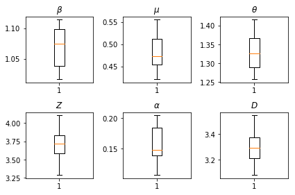
תוצאות המסקנות שלנו. אנו נצייר את ערכי המקסימום-הסבירות עבור כל paramters הגלובלית להראות וריאציה שלהם ברחבי שלנו num_batches ריצות עצמאית של היקש. זה מתאים לטבלה S1 בחומרים המשלימים.
fig, axs = plt.subplots(2, 3)
axs[0, 0].boxplot(best_parameters.documented_infectious_tx_rate,
                  whis=(2.5,97.5), sym='')
axs[0, 0].set_title(r'$\beta$')

axs[0, 1].boxplot(best_parameters.undocumented_infectious_tx_relative_rate,
                  whis=(2.5,97.5), sym='')
axs[0, 1].set_title(r'$\mu$')

axs[0, 2].boxplot(best_parameters.intercity_underreporting_factor,
                  whis=(2.5,97.5), sym='')
axs[0, 2].set_title(r'$\theta$')

axs[1, 0].boxplot(best_parameters.average_latency_period,
                  whis=(2.5,97.5), sym='')
axs[1, 0].set_title(r'$Z$')

axs[1, 1].boxplot(best_parameters.fraction_of_documented_infections,
                  whis=(2.5,97.5), sym='')
axs[1, 1].set_title(r'$\alpha$')

axs[1, 2].boxplot(best_parameters.average_infection_duration,
                  whis=(2.5,97.5), sym='')
axs[1, 2].set_title(r'$D$')
plt.tight_layout()