
| | |  Xem nguồn trên GitHub Xem nguồn trên GitHub | |
Trong ví dụ này, bạn sẽ khám phá kết quả của McClean, 2019 cho biết không chỉ bất kỳ cấu trúc mạng nơ-ron lượng tử nào cũng sẽ hoạt động tốt khi nói đến việc học. Đặc biệt, bạn sẽ thấy rằng một nhóm lớn các mạch lượng tử ngẫu nhiên không đóng vai trò là các mạng nơron lượng tử tốt, bởi vì chúng có độ dốc biến mất hầu như ở khắp mọi nơi. Trong ví dụ này, bạn sẽ không đào tạo bất kỳ mô hình nào cho một vấn đề học tập cụ thể, mà thay vào đó tập trung vào vấn đề đơn giản hơn là hiểu hành vi của các gradient.
Thành lập
pip install tensorflow==2.7.0
Cài đặt TensorFlow Quantum:
pip install tensorflow-quantum
# Update package resources to account for version changes.
import importlib, pkg_resources
importlib.reload(pkg_resources)
<module 'pkg_resources' from '/tmpfs/src/tf_docs_env/lib/python3.7/site-packages/pkg_resources/__init__.py'>
Bây giờ nhập TensorFlow và các phụ thuộc mô-đun:
import tensorflow as tf
import tensorflow_quantum as tfq

import cirq
import sympy
import numpy as np

# visualization tools
%matplotlib inline
import matplotlib.pyplot as plt
from cirq.contrib.svg import SVGCircuit

np.random.seed(1234)
2022-02-04 12:15:43.355568: E tensorflow/stream_executor/cuda/cuda_driver.cc:271] failed call to cuInit: CUDA_ERROR_NO_DEVICE: no CUDA-capable device is detected
1. Tóm tắt
Các mạch lượng tử ngẫu nhiên có nhiều khối trông giống như thế này (\(R_{P}(\theta)\) là một phép quay Pauli ngẫu nhiên):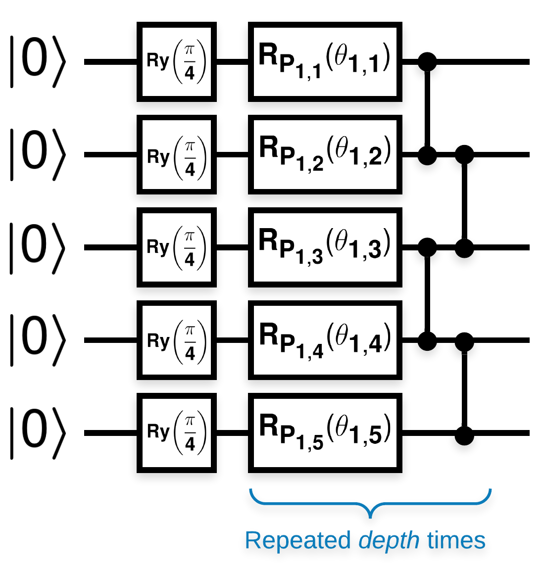
Trong đó nếu \(f(x)\) được xác định là giá trị kỳ vọng wrt \(Z_{a}Z_{b}\) cho bất kỳ qubit nào \(a\) và \(b\), thì có một vấn đề là \(f'(x)\) có giá trị trung bình rất gần với 0 và không thay đổi nhiều. Bạn sẽ thấy điều này bên dưới:
2. Tạo mạch ngẫu nhiên
Việc xây dựng từ giấy là đơn giản để làm theo. Phần sau thực hiện một chức năng đơn giản tạo ra một mạch lượng tử ngẫu nhiên — đôi khi được gọi là mạng nơ-ron lượng tử (QNN) —với độ sâu đã cho trên một tập hợp các qubit:
def generate_random_qnn(qubits, symbol, depth):
    """Generate random QNN's with the same structure from McClean et al."""
    circuit = cirq.Circuit()
    for qubit in qubits:
        circuit += cirq.ry(np.pi / 4.0)(qubit)

    for d in range(depth):
        # Add a series of single qubit rotations.
        for i, qubit in enumerate(qubits):
            random_n = np.random.uniform()
            random_rot = np.random.uniform(
            ) * 2.0 * np.pi if i != 0 or d != 0 else symbol
            if random_n > 2. / 3.:
                # Add a Z.
                circuit += cirq.rz(random_rot)(qubit)
            elif random_n > 1. / 3.:
                # Add a Y.
                circuit += cirq.ry(random_rot)(qubit)
            else:
                # Add a X.
                circuit += cirq.rx(random_rot)(qubit)

        # Add CZ ladder.
        for src, dest in zip(qubits, qubits[1:]):
            circuit += cirq.CZ(src, dest)

    return circuit


generate_random_qnn(cirq.GridQubit.rect(1, 3), sympy.Symbol('theta'), 2)
Các tác giả điều tra gradient của một tham số duy nhất \(\theta_{1,1}\). Hãy cùng theo dõi bằng cách đặt một sympy.Symbol trong mạch mà ở đó \(\theta_{1,1}\) sẽ là. Vì các tác giả không phân tích thống kê cho bất kỳ ký hiệu nào khác trong mạch, chúng ta hãy thay thế chúng bằng các giá trị ngẫu nhiên ngay bây giờ thay vì sau này.
3. Chạy các mạch
Tạo một vài trong số các mạch này cùng với một mạch có thể quan sát được để kiểm tra tuyên bố rằng độ dốc không thay đổi nhiều. Đầu tiên, tạo một loạt các mạch ngẫu nhiên. Chọn một ZZ ngẫu nhiên có thể quan sát được và tính toán hàng loạt các gradient và phương sai bằng cách sử dụng TensorFlow Quantum.
3.1 Tính toán phương sai hàng loạt
Hãy viết một hàm trợ giúp để tính toán phương sai của gradient của một khối nhất định có thể quan sát được trên một loạt mạch:
def process_batch(circuits, symbol, op):
    """Compute the variance of a batch of expectations w.r.t. op on each circuit that
    contains `symbol`. Note that this method sets up a new compute graph every time it is
    called so it isn't as performant as possible."""

    # Setup a simple layer to batch compute the expectation gradients.
    expectation = tfq.layers.Expectation()

    # Prep the inputs as tensors
    circuit_tensor = tfq.convert_to_tensor(circuits)
    values_tensor = tf.convert_to_tensor(
        np.random.uniform(0, 2 * np.pi, (n_circuits, 1)).astype(np.float32))

    # Use TensorFlow GradientTape to track gradients.
    with tf.GradientTape() as g:
        g.watch(values_tensor)
        forward = expectation(circuit_tensor,
                              operators=op,
                              symbol_names=[symbol],
                              symbol_values=values_tensor)

    # Return variance of gradients across all circuits.
    grads = g.gradient(forward, values_tensor)
    grad_var = tf.math.reduce_std(grads, axis=0)
    return grad_var.numpy()[0]
3.1 Thiết lập và chạy
Chọn số lượng mạch ngẫu nhiên để tạo ra cùng với độ sâu của chúng và số lượng qubit mà chúng phải hoạt động. Sau đó vẽ biểu đồ kết quả.
n_qubits = [2 * i for i in range(2, 7)
           ]  # Ranges studied in paper are between 2 and 24.
depth = 50  # Ranges studied in paper are between 50 and 500.
n_circuits = 200
theta_var = []

for n in n_qubits:
    # Generate the random circuits and observable for the given n.
    qubits = cirq.GridQubit.rect(1, n)
    symbol = sympy.Symbol('theta')
    circuits = [
        generate_random_qnn(qubits, symbol, depth) for _ in range(n_circuits)
    ]
    op = cirq.Z(qubits[0]) * cirq.Z(qubits[1])
    theta_var.append(process_batch(circuits, symbol, op))

plt.semilogy(n_qubits, theta_var)
plt.title('Gradient Variance in QNNs')
plt.xlabel('n_qubits')
plt.xticks(n_qubits)
plt.ylabel('$\\partial \\theta$ variance')
plt.show()
WARNING:tensorflow:5 out of the last 5 calls to <function Adjoint.differentiate_analytic at 0x7f9e3b5c68c0> triggered tf.function retracing. Tracing is expensive and the excessive number of tracings could be due to (1) creating @tf.function repeatedly in a loop, (2) passing tensors with different shapes, (3) passing Python objects instead of tensors. For (1), please define your @tf.function outside of the loop. For (2), @tf.function has experimental_relax_shapes=True option that relaxes argument shapes that can avoid unnecessary retracing. For (3), please refer to https://www.tensorflow.org/guide/function#controlling_retracing and https://www.tensorflow.org/api_docs/python/tf/function for more details.
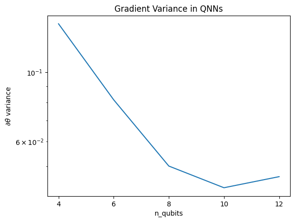
Biểu đồ này cho thấy rằng đối với các bài toán máy học lượng tử, bạn không thể đơn giản đoán một ansatz QNN ngẫu nhiên và hy vọng điều tốt nhất. Một số cấu trúc phải hiện diện trong mạch mô hình để cho các độ dốc thay đổi đến mức mà việc học có thể xảy ra.
4. Heuristics
Một kinh nghiệm thú vị của Grant, năm 2019 cho phép một người bắt đầu rất gần với ngẫu nhiên, nhưng không hoàn toàn. Sử dụng các mạch tương tự như McClean và cộng sự, các tác giả đề xuất một kỹ thuật khởi tạo khác cho các thông số điều khiển cổ điển để tránh các cao nguyên cằn cỗi. Kỹ thuật khởi tạo bắt đầu một số lớp với các tham số điều khiển hoàn toàn ngẫu nhiên — nhưng, trong các lớp ngay sau đó, hãy chọn các tham số sao cho quá trình chuyển đổi ban đầu được thực hiện bởi một vài lớp đầu tiên được hoàn tác. Các tác giả gọi đây là một khối nhận dạng .
Ưu điểm của phương pháp heuristic này là bằng cách chỉ thay đổi một tham số duy nhất, tất cả các khối khác bên ngoài khối hiện tại sẽ vẫn là danh tính — và tín hiệu gradient đi qua mạnh hơn nhiều so với trước đây. Điều này cho phép người dùng chọn và chọn các biến và khối cần sửa đổi để có được tín hiệu gradient mạnh mẽ. Kinh nghiệm này không ngăn người dùng rơi vào vùng cao nguyên cằn cỗi trong giai đoạn huấn luyện (và hạn chế cập nhật hoàn toàn đồng thời), nó chỉ đảm bảo rằng bạn có thể bắt đầu bên ngoài vùng bình nguyên.
4.1 Xây dựng QNN mới
Bây giờ hãy xây dựng một hàm để tạo ra các QNN của khối nhận dạng. Cách triển khai này hơi khác so với cách triển khai trên giấy. Hiện tại, hãy nhìn vào hoạt động của gradient của một tham số duy nhất để nó phù hợp với McClean và cộng sự, vì vậy có thể thực hiện một số đơn giản hóa.
Để tạo khối nhận dạng và đào tạo mô hình, thông thường bạn cần \(U1(\theta_{1a}) U1(\theta_{1b})^{\dagger}\) chứ không phải \(U1(\theta_1) U1(\theta_1)^{\dagger}\). Ban đầu \(\theta_{1a}\) và \(\theta_{1b}\) là các góc giống nhau nhưng chúng được học một cách độc lập. Nếu không, bạn sẽ luôn nhận được danh tính ngay cả sau khi đào tạo. Sự lựa chọn cho số lượng khối nhận dạng là theo kinh nghiệm. Khối càng sâu, phương sai ở giữa khối càng nhỏ. Nhưng ở phần đầu và phần cuối của khối, phương sai của các gradient tham số phải lớn.
def generate_identity_qnn(qubits, symbol, block_depth, total_depth):
    """Generate random QNN's with the same structure from Grant et al."""
    circuit = cirq.Circuit()

    # Generate initial block with symbol.
    prep_and_U = generate_random_qnn(qubits, symbol, block_depth)
    circuit += prep_and_U

    # Generate dagger of initial block without symbol.
    U_dagger = (prep_and_U[1:])**-1
    circuit += cirq.resolve_parameters(
        U_dagger, param_resolver={symbol: np.random.uniform() * 2 * np.pi})

    for d in range(total_depth - 1):
        # Get a random QNN.
        prep_and_U_circuit = generate_random_qnn(
            qubits,
            np.random.uniform() * 2 * np.pi, block_depth)

        # Remove the state-prep component
        U_circuit = prep_and_U_circuit[1:]

        # Add U
        circuit += U_circuit

        # Add U^dagger
        circuit += U_circuit**-1

    return circuit


generate_identity_qnn(cirq.GridQubit.rect(1, 3), sympy.Symbol('theta'), 2, 2)
4.2 So sánh
Ở đây, bạn có thể thấy rằng heuristic giúp giữ cho phương sai của gradient không biến mất nhanh chóng:
block_depth = 10
total_depth = 5

heuristic_theta_var = []

for n in n_qubits:
    # Generate the identity block circuits and observable for the given n.
    qubits = cirq.GridQubit.rect(1, n)
    symbol = sympy.Symbol('theta')
    circuits = [
        generate_identity_qnn(qubits, symbol, block_depth, total_depth)
        for _ in range(n_circuits)
    ]
    op = cirq.Z(qubits[0]) * cirq.Z(qubits[1])
    heuristic_theta_var.append(process_batch(circuits, symbol, op))

plt.semilogy(n_qubits, theta_var)
plt.semilogy(n_qubits, heuristic_theta_var)
plt.title('Heuristic vs. Random')
plt.xlabel('n_qubits')
plt.xticks(n_qubits)
plt.ylabel('$\\partial \\theta$ variance')
plt.show()
WARNING:tensorflow:6 out of the last 6 calls to <function Adjoint.differentiate_analytic at 0x7f9e3b5c68c0> triggered tf.function retracing. Tracing is expensive and the excessive number of tracings could be due to (1) creating @tf.function repeatedly in a loop, (2) passing tensors with different shapes, (3) passing Python objects instead of tensors. For (1), please define your @tf.function outside of the loop. For (2), @tf.function has experimental_relax_shapes=True option that relaxes argument shapes that can avoid unnecessary retracing. For (3), please refer to https://www.tensorflow.org/guide/function#controlling_retracing and https://www.tensorflow.org/api_docs/python/tf/function for more details.
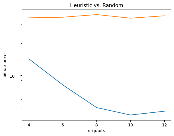
Đây là một cải tiến lớn trong việc nhận tín hiệu gradient mạnh hơn từ các QNN ngẫu nhiên (gần).