
| | |  Посмотреть исходный код на GitHub Посмотреть исходный код на GitHub | |
В этом руководстве рассматриваются алгоритмы расчета градиента для ожидаемых значений квантовых схем.
Вычисление градиента ожидаемого значения некоторой наблюдаемой в квантовой схеме — сложный процесс. Ожидаемые значения наблюдаемых не могут позволить себе роскошь иметь аналитические формулы градиента, которые всегда легко записать, в отличие от традиционных преобразований машинного обучения, таких как умножение матриц или сложение векторов, которые имеют аналитические формулы градиента, которые легко записать. В результате существуют разные методы расчета квантового градиента, которые пригодятся для разных сценариев. В этом руководстве сравниваются и противопоставляются две разные схемы дифференциации.
Настраивать
pip install tensorflow==2.7.0
Установите TensorFlow Quantum:
pip install tensorflow-quantum
# Update package resources to account for version changes.
import importlib, pkg_resources
importlib.reload(pkg_resources)
<module 'pkg_resources' from '/tmpfs/src/tf_docs_env/lib/python3.7/site-packages/pkg_resources/__init__.py'>
Теперь импортируйте TensorFlow и зависимости модуля:
import tensorflow as tf
import tensorflow_quantum as tfq

import cirq
import sympy
import numpy as np

# visualization tools
%matplotlib inline
import matplotlib.pyplot as plt
from cirq.contrib.svg import SVGCircuit
2022-02-04 12:25:24.733670: E tensorflow/stream_executor/cuda/cuda_driver.cc:271] failed call to cuInit: CUDA_ERROR_NO_DEVICE: no CUDA-capable device is detected
1. Предварительный
Давайте немного конкретизируем понятие вычисления градиента для квантовых схем. Предположим, у вас есть параметризованная схема, подобная этой:
qubit = cirq.GridQubit(0, 0)
my_circuit = cirq.Circuit(cirq.Y(qubit)**sympy.Symbol('alpha'))
SVGCircuit(my_circuit)
findfont: Font family ['Arial'] not found. Falling back to DejaVu Sans.

Наряду с наблюдаемым:
pauli_x = cirq.X(qubit)
pauli_x
cirq.X(cirq.GridQubit(0, 0))
Глядя на этот оператор, вы знаете, что \(⟨Y(\alpha)| X | Y(\alpha)⟩ = \sin(\pi \alpha)\)
def my_expectation(op, alpha):
    """Compute ⟨Y(alpha)| `op` | Y(alpha)⟩"""
    params = {'alpha': alpha}
    sim = cirq.Simulator()
    final_state_vector = sim.simulate(my_circuit, params).final_state_vector
    return op.expectation_from_state_vector(final_state_vector, {qubit: 0}).real


my_alpha = 0.3
print("Expectation=", my_expectation(pauli_x, my_alpha))
print("Sin Formula=", np.sin(np.pi * my_alpha))
Expectation= 0.80901700258255
Sin Formula= 0.8090169943749475
и если вы определяете \(f_{1}(\alpha) = ⟨Y(\alpha)| X | Y(\alpha)⟩\) то \(f_{1}^{'}(\alpha) = \pi \cos(\pi \alpha)\). Давайте проверим это:
def my_grad(obs, alpha, eps=0.01):
    grad = 0
    f_x = my_expectation(obs, alpha)
    f_x_prime = my_expectation(obs, alpha + eps)
    return ((f_x_prime - f_x) / eps).real


print('Finite difference:', my_grad(pauli_x, my_alpha))
print('Cosine formula:   ', np.pi * np.cos(np.pi * my_alpha))
Finite difference: 1.8063604831695557
Cosine formula:    1.8465818304904567
2. Потребность в отличительном признаке
С более крупными схемами вам не всегда повезет иметь формулу, которая точно вычисляет градиенты данной квантовой схемы. В случае, если простой формулы недостаточно для расчета градиента, класс tfq.differentiators.Differentiator . Differentiators.Differentiator позволяет определить алгоритмы для вычисления градиентов ваших цепей. Например, вы можете воссоздать приведенный выше пример в TensorFlow Quantum (TFQ) с помощью:
expectation_calculation = tfq.layers.Expectation(
    differentiator=tfq.differentiators.ForwardDifference(grid_spacing=0.01))

expectation_calculation(my_circuit,
                        operators=pauli_x,
                        symbol_names=['alpha'],
                        symbol_values=[[my_alpha]])
<tf.Tensor: shape=(1, 1), dtype=float32, numpy=array([[0.80901706]], dtype=float32)>
Однако, если вы переключитесь на оценку ожидания на основе выборки (что произойдет на реальном устройстве), значения могут немного измениться. Это означает, что теперь у вас есть несовершенная оценка:
sampled_expectation_calculation = tfq.layers.SampledExpectation(
    differentiator=tfq.differentiators.ForwardDifference(grid_spacing=0.01))

sampled_expectation_calculation(my_circuit,
                                operators=pauli_x,
                                repetitions=500,
                                symbol_names=['alpha'],
                                symbol_values=[[my_alpha]])
<tf.Tensor: shape=(1, 1), dtype=float32, numpy=array([[0.836]], dtype=float32)>
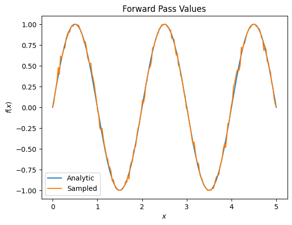
Это может быстро привести к серьезной проблеме с точностью, когда дело доходит до градиентов:
# Make input_points = [batch_size, 1] array.
input_points = np.linspace(0, 5, 200)[:, np.newaxis].astype(np.float32)
exact_outputs = expectation_calculation(my_circuit,
                                        operators=pauli_x,
                                        symbol_names=['alpha'],
                                        symbol_values=input_points)
imperfect_outputs = sampled_expectation_calculation(my_circuit,
                                                    operators=pauli_x,
                                                    repetitions=500,
                                                    symbol_names=['alpha'],
                                                    symbol_values=input_points)
plt.title('Forward Pass Values')
plt.xlabel('$x$')
plt.ylabel('$f(x)$')
plt.plot(input_points, exact_outputs, label='Analytic')
plt.plot(input_points, imperfect_outputs, label='Sampled')
plt.legend()
<matplotlib.legend.Legend at 0x7ff07d556190>
# Gradients are a much different story.
values_tensor = tf.convert_to_tensor(input_points)

with tf.GradientTape() as g:
    g.watch(values_tensor)
    exact_outputs = expectation_calculation(my_circuit,
                                            operators=pauli_x,
                                            symbol_names=['alpha'],
                                            symbol_values=values_tensor)
analytic_finite_diff_gradients = g.gradient(exact_outputs, values_tensor)

with tf.GradientTape() as g:
    g.watch(values_tensor)
    imperfect_outputs = sampled_expectation_calculation(
        my_circuit,
        operators=pauli_x,
        repetitions=500,
        symbol_names=['alpha'],
        symbol_values=values_tensor)
sampled_finite_diff_gradients = g.gradient(imperfect_outputs, values_tensor)

plt.title('Gradient Values')
plt.xlabel('$x$')
plt.ylabel('$f^{\'}(x)$')
plt.plot(input_points, analytic_finite_diff_gradients, label='Analytic')
plt.plot(input_points, sampled_finite_diff_gradients, label='Sampled')
plt.legend()
<matplotlib.legend.Legend at 0x7ff07adb8dd0>
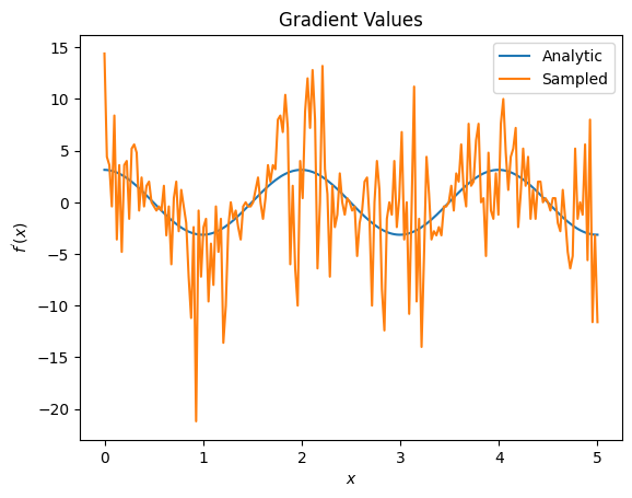
Здесь вы можете видеть, что, хотя формула конечных разностей быстро вычисляет сами градиенты в аналитическом случае, когда дело дошло до методов, основанных на выборке, она была слишком шумной. Необходимо использовать более тщательные методы, чтобы обеспечить возможность расчета хорошего градиента. Далее вы рассмотрите гораздо более медленный метод, который не так хорошо подходит для аналитических вычислений градиента ожидания, но работает намного лучше в случае, основанном на реальной выборке:
# A smarter differentiation scheme.
gradient_safe_sampled_expectation = tfq.layers.SampledExpectation(
    differentiator=tfq.differentiators.ParameterShift())

with tf.GradientTape() as g:
    g.watch(values_tensor)
    imperfect_outputs = gradient_safe_sampled_expectation(
        my_circuit,
        operators=pauli_x,
        repetitions=500,
        symbol_names=['alpha'],
        symbol_values=values_tensor)

sampled_param_shift_gradients = g.gradient(imperfect_outputs, values_tensor)

plt.title('Gradient Values')
plt.xlabel('$x$')
plt.ylabel('$f^{\'}(x)$')
plt.plot(input_points, analytic_finite_diff_gradients, label='Analytic')
plt.plot(input_points, sampled_param_shift_gradients, label='Sampled')
plt.legend()
<matplotlib.legend.Legend at 0x7ff07ad9ff90>
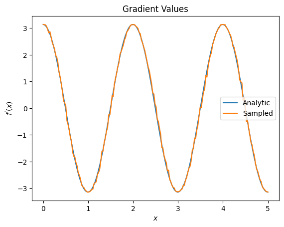
Из вышеизложенного вы можете видеть, что определенные дифференциаторы лучше всего использовать для конкретных сценариев исследования. В общем, более медленные методы на основе сэмплов, которые устойчивы к шуму устройства и т. д., являются отличными отличиями при тестировании или реализации алгоритмов в более «реальных» условиях. Более быстрые методы, такие как конечная разность, отлично подходят для аналитических вычислений, и вам нужна более высокая пропускная способность, но пока вас не беспокоит жизнеспособность вашего алгоритма на устройстве.
3. Несколько наблюдаемых
Давайте представим вторую наблюдаемую и посмотрим, как TensorFlow Quantum поддерживает несколько наблюдаемых для одной схемы.
pauli_z = cirq.Z(qubit)
pauli_z
cirq.Z(cirq.GridQubit(0, 0))
Если этот наблюдаемый используется с той же схемой, что и раньше, то у вас есть \(f_{2}(\alpha) = ⟨Y(\alpha)| Z | Y(\alpha)⟩ = \cos(\pi \alpha)\) и \(f_{2}^{'}(\alpha) = -\pi \sin(\pi \alpha)\). Выполните быструю проверку:
test_value = 0.

print('Finite difference:', my_grad(pauli_z, test_value))
print('Sin formula:      ', -np.pi * np.sin(np.pi * test_value))
Finite difference: -0.04934072494506836
Sin formula:       -0.0
Это совпадение (достаточно близкое).
Теперь, если вы определите \(g(\alpha) = f_{1}(\alpha) + f_{2}(\alpha)\) то \(g'(\alpha) = f_{1}^{'}(\alpha) + f^{'}_{2}(\alpha)\). Определение нескольких наблюдаемых в TensorFlow Quantum для использования вместе со схемой эквивалентно добавлению дополнительных терминов в \(g\).
Это означает, что градиент конкретного символа в схеме равен сумме градиентов относительно каждого наблюдаемого для этого символа, примененного к этой схеме. Это совместимо с получением градиента TensorFlow и обратным распространением (где вы задаете сумму градиентов по всем наблюдаемым в качестве градиента для определенного символа).
sum_of_outputs = tfq.layers.Expectation(
    differentiator=tfq.differentiators.ForwardDifference(grid_spacing=0.01))

sum_of_outputs(my_circuit,
               operators=[pauli_x, pauli_z],
               symbol_names=['alpha'],
               symbol_values=[[test_value]])
<tf.Tensor: shape=(1, 2), dtype=float32, numpy=array([[1.9106855e-15, 1.0000000e+00]], dtype=float32)>
Здесь вы видите, что первая запись — это ожидание относительно Паули X, а вторая — ожидание относительно Паули Z. Теперь, когда вы берете градиент:
test_value_tensor = tf.convert_to_tensor([[test_value]])

with tf.GradientTape() as g:
    g.watch(test_value_tensor)
    outputs = sum_of_outputs(my_circuit,
                             operators=[pauli_x, pauli_z],
                             symbol_names=['alpha'],
                             symbol_values=test_value_tensor)

sum_of_gradients = g.gradient(outputs, test_value_tensor)

print(my_grad(pauli_x, test_value) + my_grad(pauli_z, test_value))
print(sum_of_gradients.numpy())
3.0917350202798843
[[3.0917213]]
Здесь вы убедились, что сумма градиентов для каждой наблюдаемой действительно является градиентом \(\alpha\). Это поведение поддерживается всеми дифференциаторами TensorFlow Quantum и играет решающую роль в совместимости с остальной частью TensorFlow.
4. Расширенное использование
Все дифференциаторы, которые существуют внутри подкласса tfq.differentiators.Differentiator Quantum tfq. Differentiators.Differentiator . Чтобы реализовать дифференциатор, пользователь должен реализовать один из двух интерфейсов. Стандартом является реализация get_gradient_circuits , которая сообщает базовому классу, какие схемы нужно измерить, чтобы получить оценку градиента. В качестве альтернативы вы можете перегрузить differentiate_analytic и differentiate_sampled ; класс tfq.differentiators.Adjoint . Differentiators.Adjoint идет по этому пути.
Следующее использует TensorFlow Quantum для реализации градиента цепи. Вы будете использовать небольшой пример смещения параметра.
Вспомните схему, которую вы определили выше, \(|\alpha⟩ = Y^{\alpha}|0⟩\). Как и прежде, вы можете определить функцию как ожидаемое значение этой схемы относительно наблюдаемого l10n- \(X\) , \(f(\alpha) = ⟨\alpha|X|\alpha⟩\). Используя правила сдвига параметров , для этой схемы можно найти, что производная равна
\[\frac{\partial}{\partial \alpha} f(\alpha) = \frac{\pi}{2} f\left(\alpha + \frac{1}{2}\right) - \frac{ \pi}{2} f\left(\alpha - \frac{1}{2}\right)\]
Функция get_gradient_circuits возвращает компоненты этой производной.
class MyDifferentiator(tfq.differentiators.Differentiator):
    """A Toy differentiator for <Y^alpha | X |Y^alpha>."""

    def __init__(self):
        pass

    def get_gradient_circuits(self, programs, symbol_names, symbol_values):
        """Return circuits to compute gradients for given forward pass circuits.

        Every gradient on a quantum computer can be computed via measurements
        of transformed quantum circuits.  Here, you implement a custom gradient
        for a specific circuit.  For a real differentiator, you will need to
        implement this function in a more general way.  See the differentiator
        implementations in the TFQ library for examples.
        """

        # The two terms in the derivative are the same circuit...
        batch_programs = tf.stack([programs, programs], axis=1)

        # ... with shifted parameter values.
        shift = tf.constant(1/2)
        forward = symbol_values + shift
        backward = symbol_values - shift
        batch_symbol_values = tf.stack([forward, backward], axis=1)

        # Weights are the coefficients of the terms in the derivative.
        num_program_copies = tf.shape(batch_programs)[0]
        batch_weights = tf.tile(tf.constant([[[np.pi/2, -np.pi/2]]]),
                                [num_program_copies, 1, 1])

        # The index map simply says which weights go with which circuits.
        batch_mapper = tf.tile(
            tf.constant([[[0, 1]]]), [num_program_copies, 1, 1])

        return (batch_programs, symbol_names, batch_symbol_values,
                batch_weights, batch_mapper)
Базовый класс Differentiator использует компоненты, возвращенные из get_gradient_circuits , для вычисления производной, как в формуле сдвига параметра, которую вы видели выше. Этот новый дифференциатор теперь можно использовать с существующими объектами tfq.layer :
custom_dif = MyDifferentiator()
custom_grad_expectation = tfq.layers.Expectation(differentiator=custom_dif)

# Now let's get the gradients with finite diff.
with tf.GradientTape() as g:
    g.watch(values_tensor)
    exact_outputs = expectation_calculation(my_circuit,
                                            operators=[pauli_x],
                                            symbol_names=['alpha'],
                                            symbol_values=values_tensor)

analytic_finite_diff_gradients = g.gradient(exact_outputs, values_tensor)

# Now let's get the gradients with custom diff.
with tf.GradientTape() as g:
    g.watch(values_tensor)
    my_outputs = custom_grad_expectation(my_circuit,
                                         operators=[pauli_x],
                                         symbol_names=['alpha'],
                                         symbol_values=values_tensor)

my_gradients = g.gradient(my_outputs, values_tensor)

plt.subplot(1, 2, 1)
plt.title('Exact Gradient')
plt.plot(input_points, analytic_finite_diff_gradients.numpy())
plt.xlabel('x')
plt.ylabel('f(x)')
plt.subplot(1, 2, 2)
plt.title('My Gradient')
plt.plot(input_points, my_gradients.numpy())
plt.xlabel('x')
Text(0.5, 0, 'x')
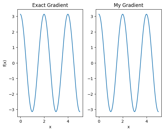
Этот новый дифференциатор теперь можно использовать для создания дифференцируемых операций.
# Create a noisy sample based expectation op.
expectation_sampled = tfq.get_sampled_expectation_op(
    cirq.DensityMatrixSimulator(noise=cirq.depolarize(0.01)))

# Make it differentiable with your differentiator:
# Remember to refresh the differentiator before attaching the new op
custom_dif.refresh()
differentiable_op = custom_dif.generate_differentiable_op(
    sampled_op=expectation_sampled)

# Prep op inputs.
circuit_tensor = tfq.convert_to_tensor([my_circuit])
op_tensor = tfq.convert_to_tensor([[pauli_x]])
single_value = tf.convert_to_tensor([[my_alpha]])
num_samples_tensor = tf.convert_to_tensor([[5000]])

with tf.GradientTape() as g:
    g.watch(single_value)
    forward_output = differentiable_op(circuit_tensor, ['alpha'], single_value,
                                       op_tensor, num_samples_tensor)

my_gradients = g.gradient(forward_output, single_value)

print('---TFQ---')
print('Foward:  ', forward_output.numpy())
print('Gradient:', my_gradients.numpy())
print('---Original---')
print('Forward: ', my_expectation(pauli_x, my_alpha))
print('Gradient:', my_grad(pauli_x, my_alpha))
---TFQ---
Foward:   [[0.8016]]
Gradient: [[1.7932211]]
---Original---
Forward:  0.80901700258255
Gradient: 1.8063604831695557