
| | |  Xem nguồn trên GitHub Xem nguồn trên GitHub | |
Hướng dẫn này khám phá các thuật toán tính toán độ dốc cho các giá trị kỳ vọng của mạch lượng tử.
Tính toán gradient của giá trị kỳ vọng của một vật nào đó có thể quan sát được trong mạch lượng tử là một quá trình có liên quan. Các giá trị kỳ vọng của các vật thể quan sát không được xa xỉ bằng việc có các công thức gradient phân tích luôn dễ dàng viết ra — không giống như các phép biến đổi học máy truyền thống như phép nhân ma trận hoặc phép cộng vectơ có các công thức gradient phân tích dễ viết ra. Do đó, có nhiều phương pháp tính toán gradient lượng tử khác nhau có ích cho các tình huống khác nhau. Hướng dẫn này so sánh và đối chiếu hai sơ đồ phân biệt khác nhau.
Thành lập
pip install tensorflow==2.7.0
Cài đặt TensorFlow Quantum:
pip install tensorflow-quantum
# Update package resources to account for version changes.
import importlib, pkg_resources
importlib.reload(pkg_resources)
<module 'pkg_resources' from '/tmpfs/src/tf_docs_env/lib/python3.7/site-packages/pkg_resources/__init__.py'>
Bây giờ nhập TensorFlow và các phụ thuộc mô-đun:
import tensorflow as tf
import tensorflow_quantum as tfq

import cirq
import sympy
import numpy as np

# visualization tools
%matplotlib inline
import matplotlib.pyplot as plt
from cirq.contrib.svg import SVGCircuit
2022-02-04 12:25:24.733670: E tensorflow/stream_executor/cuda/cuda_driver.cc:271] failed call to cuInit: CUDA_ERROR_NO_DEVICE: no CUDA-capable device is detected
1. Sơ bộ
Hãy làm cho khái niệm tính toán gradient cho các mạch lượng tử cụ thể hơn một chút. Giả sử bạn có một mạch được tham số hóa như sau:
qubit = cirq.GridQubit(0, 0)
my_circuit = cirq.Circuit(cirq.Y(qubit)**sympy.Symbol('alpha'))
SVGCircuit(my_circuit)
findfont: Font family ['Arial'] not found. Falling back to DejaVu Sans.

Cùng với một quan sát được:
pauli_x = cirq.X(qubit)
pauli_x
cirq.X(cirq.GridQubit(0, 0))
Nhìn vào toán tử này, bạn biết rằng \(⟨Y(\alpha)| X | Y(\alpha)⟩ = \sin(\pi \alpha)\)
def my_expectation(op, alpha):
    """Compute ⟨Y(alpha)| `op` | Y(alpha)⟩"""
    params = {'alpha': alpha}
    sim = cirq.Simulator()
    final_state_vector = sim.simulate(my_circuit, params).final_state_vector
    return op.expectation_from_state_vector(final_state_vector, {qubit: 0}).real


my_alpha = 0.3
print("Expectation=", my_expectation(pauli_x, my_alpha))
print("Sin Formula=", np.sin(np.pi * my_alpha))
Expectation= 0.80901700258255
Sin Formula= 0.8090169943749475
và nếu bạn xác định \(f_{1}(\alpha) = ⟨Y(\alpha)| X | Y(\alpha)⟩\) thì \(f_{1}^{'}(\alpha) = \pi \cos(\pi \alpha)\). Hãy kiểm tra điều này:
def my_grad(obs, alpha, eps=0.01):
    grad = 0
    f_x = my_expectation(obs, alpha)
    f_x_prime = my_expectation(obs, alpha + eps)
    return ((f_x_prime - f_x) / eps).real


print('Finite difference:', my_grad(pauli_x, my_alpha))
print('Cosine formula:   ', np.pi * np.cos(np.pi * my_alpha))
Finite difference: 1.8063604831695557
Cosine formula:    1.8465818304904567
2. Sự cần thiết của một sự khác biệt
Với các mạch lớn hơn, không phải lúc nào bạn cũng may mắn có được một công thức tính toán chính xác độ dốc của một mạch lượng tử nhất định. Trong trường hợp một công thức đơn giản không đủ để tính toán gradient, lớp tfq.differentiators.Differentiator cho phép bạn xác định các thuật toán để tính toán gradient của mạch của bạn. Ví dụ: bạn có thể tạo lại ví dụ trên trong TensorFlow Quantum (TFQ) với:
expectation_calculation = tfq.layers.Expectation(
    differentiator=tfq.differentiators.ForwardDifference(grid_spacing=0.01))

expectation_calculation(my_circuit,
                        operators=pauli_x,
                        symbol_names=['alpha'],
                        symbol_values=[[my_alpha]])
<tf.Tensor: shape=(1, 1), dtype=float32, numpy=array([[0.80901706]], dtype=float32)>
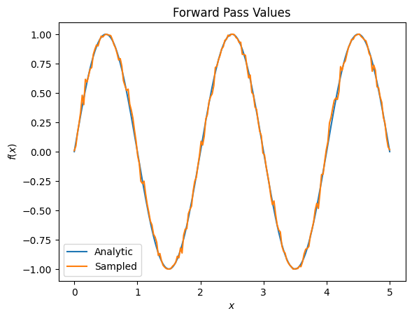
Tuy nhiên, nếu bạn chuyển sang ước tính kỳ vọng dựa trên lấy mẫu (điều gì sẽ xảy ra trên một thiết bị thực) thì các giá trị có thể thay đổi một chút. Điều này có nghĩa là bây giờ bạn có một ước tính không hoàn hảo:
sampled_expectation_calculation = tfq.layers.SampledExpectation(
    differentiator=tfq.differentiators.ForwardDifference(grid_spacing=0.01))

sampled_expectation_calculation(my_circuit,
                                operators=pauli_x,
                                repetitions=500,
                                symbol_names=['alpha'],
                                symbol_values=[[my_alpha]])
<tf.Tensor: shape=(1, 1), dtype=float32, numpy=array([[0.836]], dtype=float32)>
Điều này có thể nhanh chóng trở thành một vấn đề nghiêm trọng về độ chính xác khi nói đến độ dốc:
# Make input_points = [batch_size, 1] array.
input_points = np.linspace(0, 5, 200)[:, np.newaxis].astype(np.float32)
exact_outputs = expectation_calculation(my_circuit,
                                        operators=pauli_x,
                                        symbol_names=['alpha'],
                                        symbol_values=input_points)
imperfect_outputs = sampled_expectation_calculation(my_circuit,
                                                    operators=pauli_x,
                                                    repetitions=500,
                                                    symbol_names=['alpha'],
                                                    symbol_values=input_points)
plt.title('Forward Pass Values')
plt.xlabel('$x$')
plt.ylabel('$f(x)$')
plt.plot(input_points, exact_outputs, label='Analytic')
plt.plot(input_points, imperfect_outputs, label='Sampled')
plt.legend()
<matplotlib.legend.Legend at 0x7ff07d556190>
# Gradients are a much different story.
values_tensor = tf.convert_to_tensor(input_points)

with tf.GradientTape() as g:
    g.watch(values_tensor)
    exact_outputs = expectation_calculation(my_circuit,
                                            operators=pauli_x,
                                            symbol_names=['alpha'],
                                            symbol_values=values_tensor)
analytic_finite_diff_gradients = g.gradient(exact_outputs, values_tensor)

with tf.GradientTape() as g:
    g.watch(values_tensor)
    imperfect_outputs = sampled_expectation_calculation(
        my_circuit,
        operators=pauli_x,
        repetitions=500,
        symbol_names=['alpha'],
        symbol_values=values_tensor)
sampled_finite_diff_gradients = g.gradient(imperfect_outputs, values_tensor)

plt.title('Gradient Values')
plt.xlabel('$x$')
plt.ylabel('$f^{\'}(x)$')
plt.plot(input_points, analytic_finite_diff_gradients, label='Analytic')
plt.plot(input_points, sampled_finite_diff_gradients, label='Sampled')
plt.legend()
<matplotlib.legend.Legend at 0x7ff07adb8dd0>
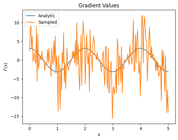
Ở đây bạn có thể thấy rằng mặc dù công thức sai phân hữu hạn nhanh chóng tự tính toán các gradient trong trường hợp phân tích, nhưng khi nói đến các phương pháp dựa trên lấy mẫu, nó quá ồn ào. Các kỹ thuật cẩn thận hơn phải được sử dụng để đảm bảo có thể tính được độ dốc tốt. Tiếp theo, bạn sẽ xem xét một kỹ thuật chậm hơn nhiều sẽ không phù hợp cho các tính toán gradient kỳ vọng phân tích, nhưng hoạt động tốt hơn nhiều trong trường hợp dựa trên mẫu trong thế giới thực:
# A smarter differentiation scheme.
gradient_safe_sampled_expectation = tfq.layers.SampledExpectation(
    differentiator=tfq.differentiators.ParameterShift())

with tf.GradientTape() as g:
    g.watch(values_tensor)
    imperfect_outputs = gradient_safe_sampled_expectation(
        my_circuit,
        operators=pauli_x,
        repetitions=500,
        symbol_names=['alpha'],
        symbol_values=values_tensor)

sampled_param_shift_gradients = g.gradient(imperfect_outputs, values_tensor)

plt.title('Gradient Values')
plt.xlabel('$x$')
plt.ylabel('$f^{\'}(x)$')
plt.plot(input_points, analytic_finite_diff_gradients, label='Analytic')
plt.plot(input_points, sampled_param_shift_gradients, label='Sampled')
plt.legend()
<matplotlib.legend.Legend at 0x7ff07ad9ff90>
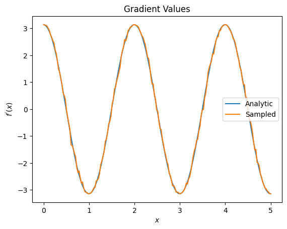
Từ những điều trên, bạn có thể thấy rằng một số yếu tố khác biệt nhất định được sử dụng tốt nhất cho các tình huống nghiên cứu cụ thể. Nói chung, các phương pháp dựa trên mẫu chậm hơn nhưng chắc chắn với nhiễu thiết bị, v.v. là những yếu tố khác biệt tuyệt vời khi thử nghiệm hoặc triển khai các thuật toán trong một cài đặt "thế giới thực" hơn. Các phương pháp nhanh hơn như sự khác biệt hữu hạn là rất tốt cho các tính toán phân tích và bạn muốn thông lượng cao hơn, nhưng chưa quan tâm đến khả năng tồn tại của thiết bị trong thuật toán của bạn.
3. Nhiều khả năng quan sát
Hãy giới thiệu một thứ hai có thể quan sát và xem cách TensorFlow Quantum hỗ trợ nhiều khả năng quan sát cho một mạch đơn lẻ.
pauli_z = cirq.Z(qubit)
pauli_z
cirq.Z(cirq.GridQubit(0, 0))
Nếu có thể quan sát được này được sử dụng với cùng một mạch như trước, thì bạn có \(f_{2}(\alpha) = ⟨Y(\alpha)| Z | Y(\alpha)⟩ = \cos(\pi \alpha)\) và \(f_{2}^{'}(\alpha) = -\pi \sin(\pi \alpha)\). Thực hiện kiểm tra nhanh:
test_value = 0.

print('Finite difference:', my_grad(pauli_z, test_value))
print('Sin formula:      ', -np.pi * np.sin(np.pi * test_value))
Finite difference: -0.04934072494506836
Sin formula:       -0.0
Đó là một trận đấu (đủ gần).
Bây giờ nếu bạn xác định \(g(\alpha) = f_{1}(\alpha) + f_{2}(\alpha)\) thì \(g'(\alpha) = f_{1}^{'}(\alpha) + f^{'}_{2}(\alpha)\). Việc xác định nhiều hơn một trong TensorFlow Quantum có thể quan sát được để sử dụng cùng với một mạch tương đương với việc thêm nhiều thuật ngữ hơn vào \(g\).
Điều này có nghĩa là gradient của một ký hiệu cụ thể trong một mạch bằng tổng của các gradient liên quan đến mỗi ký hiệu có thể quan sát được áp dụng cho mạch đó. Điều này tương thích với lấy gradient TensorFlow và lan truyền ngược (trong đó bạn cung cấp tổng các gradient trên tất cả các vật có thể quan sát làm gradient cho một biểu tượng cụ thể).
sum_of_outputs = tfq.layers.Expectation(
    differentiator=tfq.differentiators.ForwardDifference(grid_spacing=0.01))

sum_of_outputs(my_circuit,
               operators=[pauli_x, pauli_z],
               symbol_names=['alpha'],
               symbol_values=[[test_value]])
<tf.Tensor: shape=(1, 2), dtype=float32, numpy=array([[1.9106855e-15, 1.0000000e+00]], dtype=float32)>
Ở đây bạn thấy mục nhập đầu tiên là wrt Pauli X kỳ vọng và mục thứ hai là kỳ vọng wrt Pauli Z. Bây giờ khi bạn lấy gradient:
test_value_tensor = tf.convert_to_tensor([[test_value]])

with tf.GradientTape() as g:
    g.watch(test_value_tensor)
    outputs = sum_of_outputs(my_circuit,
                             operators=[pauli_x, pauli_z],
                             symbol_names=['alpha'],
                             symbol_values=test_value_tensor)

sum_of_gradients = g.gradient(outputs, test_value_tensor)

print(my_grad(pauli_x, test_value) + my_grad(pauli_z, test_value))
print(sum_of_gradients.numpy())
3.0917350202798843
[[3.0917213]]
Ở đây, bạn đã xác minh rằng tổng các gradient cho mỗi phần có thể quan sát được thực sự là gradient của \(\alpha\). Hành vi này được hỗ trợ bởi tất cả các bộ phân biệt Lượng tử TensorFlow và đóng một vai trò quan trọng trong khả năng tương thích với phần còn lại của TensorFlow.
4. Sử dụng nâng cao
Tất cả các yếu tố khác biệt tồn tại bên trong lớp con TensorFlow Quantum tfq.differentiators.Differentiator . Để triển khai một bộ phân biệt, người dùng phải triển khai một trong hai giao diện. Tiêu chuẩn là triển khai get_gradient_circuits , cho lớp cơ sở biết mạch nào cần đo để có được ước tính về gradient. Ngoài ra, bạn có thể làm quá tải phân tích differentiate_analytic và differentiate_sampled tích mẫu phân tích; lớp tfq.differentiators.Adjoint đi theo tuyến này.
Phần sau sử dụng TensorFlow Quantum để triển khai gradient của mạch. Bạn sẽ sử dụng một ví dụ nhỏ về chuyển đổi tham số.
Nhớ lại mạch bạn đã xác định ở trên, \(|\alpha⟩ = Y^{\alpha}|0⟩\). Như trước đây, bạn có thể xác định một hàm làm giá trị kỳ vọng của mạch này so với \(X\) có thể quan sát được, \(f(\alpha) = ⟨\alpha|X|\alpha⟩\). Sử dụng quy tắc dịch chuyển tham số , đối với mạch này, bạn có thể thấy rằng đạo hàm là
\[\frac{\partial}{\partial \alpha} f(\alpha) = \frac{\pi}{2} f\left(\alpha + \frac{1}{2}\right) - \frac{ \pi}{2} f\left(\alpha - \frac{1}{2}\right)\]
Hàm get_gradient_circuits trả về các thành phần của đạo hàm này.
class MyDifferentiator(tfq.differentiators.Differentiator):
    """A Toy differentiator for <Y^alpha | X |Y^alpha>."""

    def __init__(self):
        pass

    def get_gradient_circuits(self, programs, symbol_names, symbol_values):
        """Return circuits to compute gradients for given forward pass circuits.

        Every gradient on a quantum computer can be computed via measurements
        of transformed quantum circuits.  Here, you implement a custom gradient
        for a specific circuit.  For a real differentiator, you will need to
        implement this function in a more general way.  See the differentiator
        implementations in the TFQ library for examples.
        """

        # The two terms in the derivative are the same circuit...
        batch_programs = tf.stack([programs, programs], axis=1)

        # ... with shifted parameter values.
        shift = tf.constant(1/2)
        forward = symbol_values + shift
        backward = symbol_values - shift
        batch_symbol_values = tf.stack([forward, backward], axis=1)

        # Weights are the coefficients of the terms in the derivative.
        num_program_copies = tf.shape(batch_programs)[0]
        batch_weights = tf.tile(tf.constant([[[np.pi/2, -np.pi/2]]]),
                                [num_program_copies, 1, 1])

        # The index map simply says which weights go with which circuits.
        batch_mapper = tf.tile(
            tf.constant([[[0, 1]]]), [num_program_copies, 1, 1])

        return (batch_programs, symbol_names, batch_symbol_values,
                batch_weights, batch_mapper)
Lớp cơ sở Differentiator sử dụng các thành phần được trả về từ get_gradient_circuits để tính đạo hàm, như trong công thức dịch chuyển tham số mà bạn đã thấy ở trên. Công cụ phân biệt mới này hiện có thể được sử dụng với các đối tượng tfq.layer hiện có:
custom_dif = MyDifferentiator()
custom_grad_expectation = tfq.layers.Expectation(differentiator=custom_dif)

# Now let's get the gradients with finite diff.
with tf.GradientTape() as g:
    g.watch(values_tensor)
    exact_outputs = expectation_calculation(my_circuit,
                                            operators=[pauli_x],
                                            symbol_names=['alpha'],
                                            symbol_values=values_tensor)

analytic_finite_diff_gradients = g.gradient(exact_outputs, values_tensor)

# Now let's get the gradients with custom diff.
with tf.GradientTape() as g:
    g.watch(values_tensor)
    my_outputs = custom_grad_expectation(my_circuit,
                                         operators=[pauli_x],
                                         symbol_names=['alpha'],
                                         symbol_values=values_tensor)

my_gradients = g.gradient(my_outputs, values_tensor)

plt.subplot(1, 2, 1)
plt.title('Exact Gradient')
plt.plot(input_points, analytic_finite_diff_gradients.numpy())
plt.xlabel('x')
plt.ylabel('f(x)')
plt.subplot(1, 2, 2)
plt.title('My Gradient')
plt.plot(input_points, my_gradients.numpy())
plt.xlabel('x')
Text(0.5, 0, 'x')
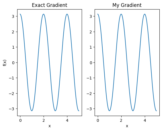
Công cụ phân biệt mới này hiện có thể được sử dụng để tạo ra các hoạt động khác biệt.
# Create a noisy sample based expectation op.
expectation_sampled = tfq.get_sampled_expectation_op(
    cirq.DensityMatrixSimulator(noise=cirq.depolarize(0.01)))

# Make it differentiable with your differentiator:
# Remember to refresh the differentiator before attaching the new op
custom_dif.refresh()
differentiable_op = custom_dif.generate_differentiable_op(
    sampled_op=expectation_sampled)

# Prep op inputs.
circuit_tensor = tfq.convert_to_tensor([my_circuit])
op_tensor = tfq.convert_to_tensor([[pauli_x]])
single_value = tf.convert_to_tensor([[my_alpha]])
num_samples_tensor = tf.convert_to_tensor([[5000]])

with tf.GradientTape() as g:
    g.watch(single_value)
    forward_output = differentiable_op(circuit_tensor, ['alpha'], single_value,
                                       op_tensor, num_samples_tensor)

my_gradients = g.gradient(forward_output, single_value)

print('---TFQ---')
print('Foward:  ', forward_output.numpy())
print('Gradient:', my_gradients.numpy())
print('---Original---')
print('Forward: ', my_expectation(pauli_x, my_alpha))
print('Gradient:', my_grad(pauli_x, my_alpha))
---TFQ---
Foward:   [[0.8016]]
Gradient: [[1.7932211]]
---Original---
Forward:  0.80901700258255
Gradient: 1.8063604831695557