TensorFlow kembali hadir di Google I/O pada 14 Mei! Daftar sekarang

Halaman ini diterjemahkan oleh Cloud Translation API.

Jaringan Saraf Konvolusi Kuantum

Lihat di TensorFlow.org

Jalankan di Google Colab

Lihat sumber di GitHub

Unduh buku catatan

Tutorial ini mengimplementasikan Quantum Convolutional Neural Network (QCNN) yang disederhanakan, analog kuantum yang diusulkan ke jaringan saraf convolutional klasik yang juga invarian translasi .

Contoh ini menunjukkan cara mendeteksi properti tertentu dari sumber data kuantum, seperti sensor kuantum atau simulasi kompleks dari perangkat. Sumber data kuantum menjadi status cluster yang mungkin atau mungkin tidak memiliki eksitasi—apa yang akan dipelajari oleh QCNN untuk dideteksi (Dataset yang digunakan dalam makalah ini adalah klasifikasi fase SPT).

Mempersiapkan

pip install tensorflow==2.7.0

Instal TensorFlow Quantum:

pip install tensorflow-quantum

# Update package resources to account for version changes.
import importlib, pkg_resources
importlib.reload(pkg_resources)

<module 'pkg_resources' from '/tmpfs/src/tf_docs_env/lib/python3.7/site-packages/pkg_resources/__init__.py'>

Sekarang impor TensorFlow dan dependensi modul:

import tensorflow as tf
import tensorflow_quantum as tfq

import cirq
import sympy
import numpy as np

# visualization tools
%matplotlib inline
import matplotlib.pyplot as plt
from cirq.contrib.svg import SVGCircuit

2022-02-04 12:43:45.380301: E tensorflow/stream_executor/cuda/cuda_driver.cc:271] failed call to cuInit: CUDA_ERROR_NO_DEVICE: no CUDA-capable device is detected

1. Bangun QCNN

1.1 Merakit sirkuit dalam grafik TensorFlow

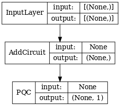
TensorFlow Quantum (TFQ) menyediakan kelas lapisan yang dirancang untuk konstruksi sirkuit dalam grafik. Salah satu contohnya adalah lapisan tfq.layers.AddCircuit yang diturunkan dari tf.keras.Layer . Lapisan ini dapat menambahkan atau menambahkan ke kumpulan input sirkuit, seperti yang ditunjukkan pada gambar berikut.

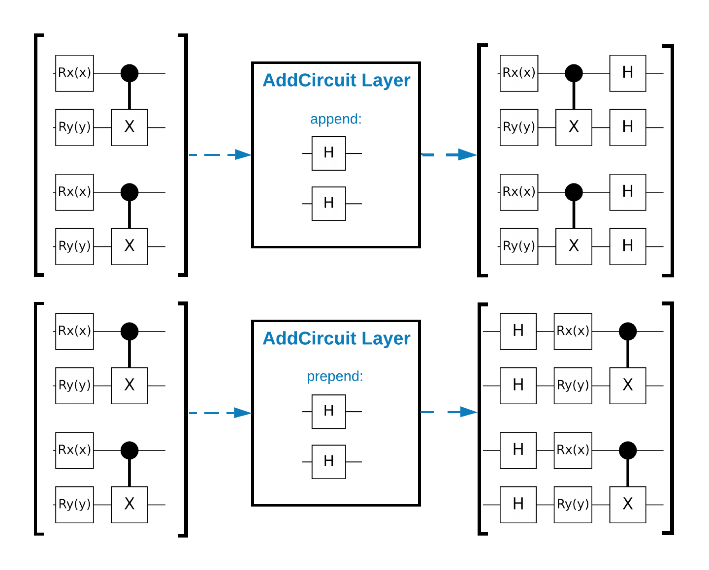
Cuplikan berikut menggunakan lapisan ini:

qubit = cirq.GridQubit(0, 0)

# Define some circuits.
circuit1 = cirq.Circuit(cirq.X(qubit))
circuit2 = cirq.Circuit(cirq.H(qubit))

# Convert to a tensor.
input_circuit_tensor = tfq.convert_to_tensor([circuit1, circuit2])

# Define a circuit that we want to append
y_circuit = cirq.Circuit(cirq.Y(qubit))

# Instantiate our layer
y_appender = tfq.layers.AddCircuit()

# Run our circuit tensor through the layer and save the output.
output_circuit_tensor = y_appender(input_circuit_tensor, append=y_circuit)

Periksa tensor input:

print(tfq.from_tensor(input_circuit_tensor))

[cirq.Circuit([
     cirq.Moment(
         cirq.X(cirq.GridQubit(0, 0)),
     ),
 ])
 cirq.Circuit([
     cirq.Moment(
         cirq.H(cirq.GridQubit(0, 0)),
     ),
 ])                                   ]

Dan periksa tensor keluaran:

print(tfq.from_tensor(output_circuit_tensor))

[cirq.Circuit([
     cirq.Moment(
         cirq.X(cirq.GridQubit(0, 0)),
     ),
     cirq.Moment(
         cirq.Y(cirq.GridQubit(0, 0)),
     ),
 ])
 cirq.Circuit([
     cirq.Moment(
         cirq.H(cirq.GridQubit(0, 0)),
     ),
     cirq.Moment(
         cirq.Y(cirq.GridQubit(0, 0)),
     ),
 ])                                   ]

Meskipun dimungkinkan untuk menjalankan contoh di bawah tanpa menggunakan tfq.layers.AddCircuit , ini adalah kesempatan yang baik untuk memahami bagaimana fungsionalitas kompleks dapat disematkan ke dalam grafik komputasi TensorFlow.

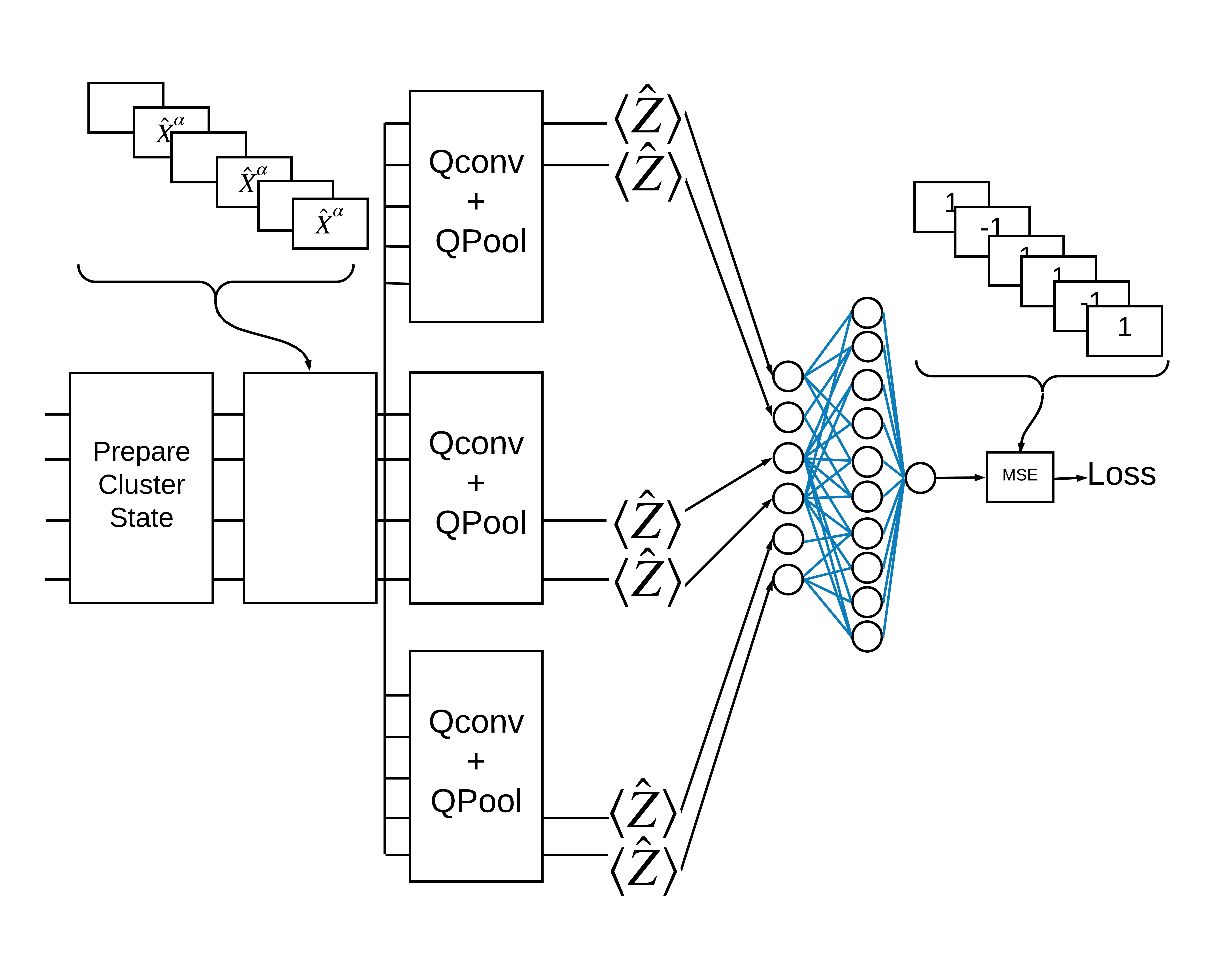
1.2 Ikhtisar masalah

Anda akan menyiapkan status klaster dan melatih pengklasifikasi kuantum untuk mendeteksi apakah "bersemangat" atau tidak. Status cluster sangat terjerat tetapi tidak selalu sulit untuk komputer klasik. Untuk kejelasan, ini adalah kumpulan data yang lebih sederhana daripada yang digunakan dalam makalah ini.

Untuk tugas klasifikasi ini, Anda akan menerapkan arsitektur QCNN mirip MERA yang dalam karena:

Seperti QCNN, status klaster pada cincin adalah invarian translasi.
Status cluster sangat terjerat.

Arsitektur ini harus efektif dalam mengurangi keterjeratan, memperoleh klasifikasi dengan membacakan satu qubit.

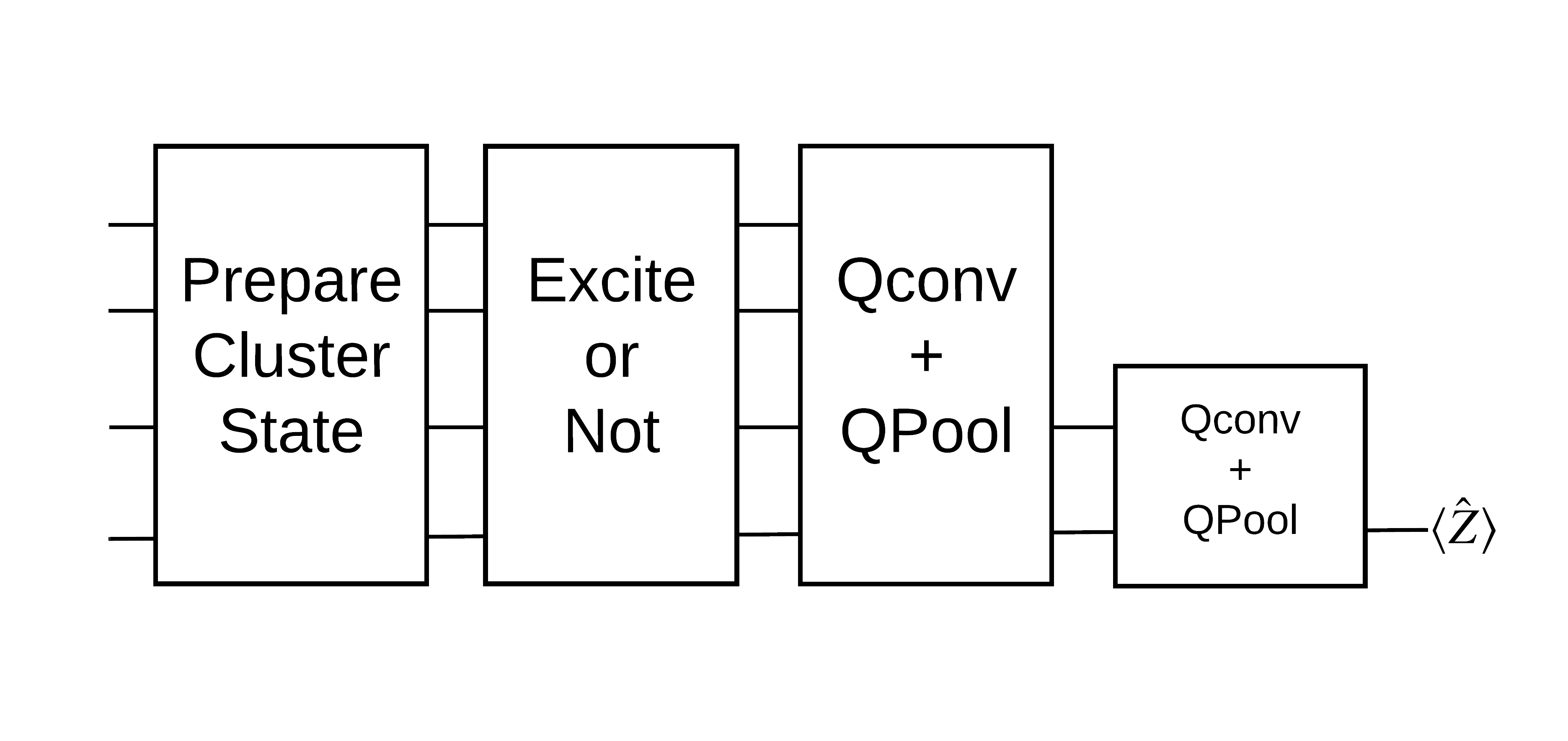
Status cluster "bersemangat" didefinisikan sebagai status cluster yang memiliki gerbang cirq.rx yang diterapkan ke salah satu qubitnya. Qconv dan QPool dibahas nanti dalam tutorial ini.

1.3 Blok penyusun untuk TensorFlow

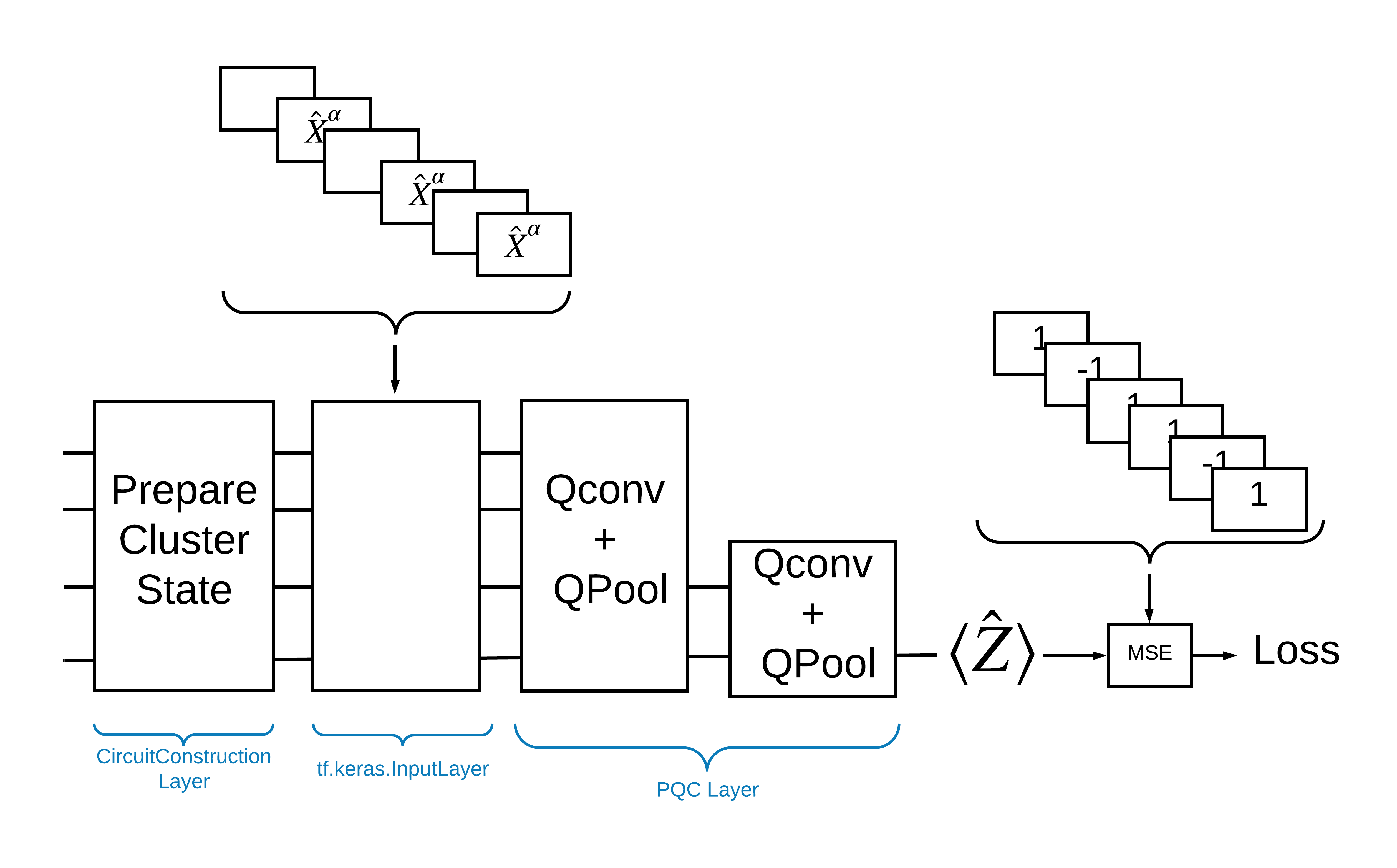
Salah satu cara untuk mengatasi masalah ini dengan TensorFlow Quantum adalah dengan menerapkan hal berikut:

Input ke model adalah tensor sirkuit—sirkuit kosong atau gerbang X pada qubit tertentu yang menunjukkan eksitasi.
Komponen kuantum model lainnya dibangun dengan lapisan tfq.layers.AddCircuit .
Untuk inferensi lapisan tfq.layers.PQC digunakan. Ini membaca \(\langle \hat{Z} \rangle\) dan membandingkannya dengan label 1 untuk keadaan tereksitasi, atau -1 untuk keadaan tidak tereksitasi.

1.4 Data

Sebelum membangun model Anda, Anda dapat menghasilkan data Anda. Dalam hal ini akan menjadi eksitasi ke status cluster (Makalah asli menggunakan dataset yang lebih rumit). Eksitasi diwakili dengan gerbang cirq.rx Putaran yang cukup besar dianggap eksitasi dan diberi label 1 dan putaran yang tidak cukup besar diberi label -1 dan dianggap bukan eksitasi.

def generate_data(qubits):
    """Generate training and testing data."""
    n_rounds = 20  # Produces n_rounds * n_qubits datapoints.
    excitations = []
    labels = []
    for n in range(n_rounds):
        for bit in qubits:
            rng = np.random.uniform(-np.pi, np.pi)
            excitations.append(cirq.Circuit(cirq.rx(rng)(bit)))
            labels.append(1 if (-np.pi / 2) <= rng <= (np.pi / 2) else -1)

    split_ind = int(len(excitations) * 0.7)
    train_excitations = excitations[:split_ind]
    test_excitations = excitations[split_ind:]

    train_labels = labels[:split_ind]
    test_labels = labels[split_ind:]

    return tfq.convert_to_tensor(train_excitations), np.array(train_labels), \
        tfq.convert_to_tensor(test_excitations), np.array(test_labels)

Anda dapat melihat bahwa seperti halnya pembelajaran mesin biasa, Anda membuat set pelatihan dan pengujian untuk digunakan sebagai tolok ukur model. Anda dapat dengan cepat melihat beberapa titik data dengan:

sample_points, sample_labels, _, __ = generate_data(cirq.GridQubit.rect(1, 4))
print('Input:', tfq.from_tensor(sample_points)[0], 'Output:', sample_labels[0])
print('Input:', tfq.from_tensor(sample_points)[1], 'Output:', sample_labels[1])

Input: (0, 0): ───X^0.449─── Output: 1
Input: (0, 1): ───X^-0.74─── Output: -1

1.5 Tentukan lapisan

Sekarang tentukan layer yang ditunjukkan pada gambar di atas di TensorFlow.

1.5.1 Status kluster

Langkah pertama adalah menentukan status cluster menggunakan Cirq , kerangka kerja yang disediakan Google untuk memprogram sirkuit kuantum. Karena ini adalah bagian statis dari model, sematkan menggunakan fungsionalitas tfq.layers.AddCircuit .

def cluster_state_circuit(bits):
    """Return a cluster state on the qubits in `bits`."""
    circuit = cirq.Circuit()
    circuit.append(cirq.H.on_each(bits))
    for this_bit, next_bit in zip(bits, bits[1:] + [bits[0]]):
        circuit.append(cirq.CZ(this_bit, next_bit))
    return circuit

Tampilkan sirkuit status cluster untuk persegi panjang dari cirq.GridQubit s:

SVGCircuit(cluster_state_circuit(cirq.GridQubit.rect(1, 4)))

findfont: Font family ['Arial'] not found. Falling back to DejaVu Sans.

svg

1.5.2 lapisan QCNN

Tentukan lapisan yang membentuk model menggunakan kertas QCNN Cong dan Lukin . Ada beberapa prasyarat:

Matriks kesatuan berparameter satu dan dua qubit dari kertas Tucci .
Operasi pengumpulan dua-qubit berparameter umum.

def one_qubit_unitary(bit, symbols):
    """Make a Cirq circuit enacting a rotation of the bloch sphere about the X,
    Y and Z axis, that depends on the values in `symbols`.
    """
    return cirq.Circuit(
        cirq.X(bit)**symbols[0],
        cirq.Y(bit)**symbols[1],
        cirq.Z(bit)**symbols[2])


def two_qubit_unitary(bits, symbols):
    """Make a Cirq circuit that creates an arbitrary two qubit unitary."""
    circuit = cirq.Circuit()
    circuit += one_qubit_unitary(bits[0], symbols[0:3])
    circuit += one_qubit_unitary(bits[1], symbols[3:6])
    circuit += [cirq.ZZ(*bits)**symbols[6]]
    circuit += [cirq.YY(*bits)**symbols[7]]
    circuit += [cirq.XX(*bits)**symbols[8]]
    circuit += one_qubit_unitary(bits[0], symbols[9:12])
    circuit += one_qubit_unitary(bits[1], symbols[12:])
    return circuit


def two_qubit_pool(source_qubit, sink_qubit, symbols):
    """Make a Cirq circuit to do a parameterized 'pooling' operation, which
    attempts to reduce entanglement down from two qubits to just one."""
    pool_circuit = cirq.Circuit()
    sink_basis_selector = one_qubit_unitary(sink_qubit, symbols[0:3])
    source_basis_selector = one_qubit_unitary(source_qubit, symbols[3:6])
    pool_circuit.append(sink_basis_selector)
    pool_circuit.append(source_basis_selector)
    pool_circuit.append(cirq.CNOT(control=source_qubit, target=sink_qubit))
    pool_circuit.append(sink_basis_selector**-1)
    return pool_circuit

Untuk melihat apa yang Anda buat, cetak sirkuit kesatuan satu-qubit:

SVGCircuit(one_qubit_unitary(cirq.GridQubit(0, 0), sympy.symbols('x0:3')))

svg

Dan sirkuit kesatuan dua-qubit:

SVGCircuit(two_qubit_unitary(cirq.GridQubit.rect(1, 2), sympy.symbols('x0:15')))

svg

Dan sirkuit penyatuan dua-qubit:

SVGCircuit(two_qubit_pool(*cirq.GridQubit.rect(1, 2), sympy.symbols('x0:6')))

svg

1.5.2.1 Konvolusi kuantum

Seperti dalam makalah Cong dan Lukin , definisikan konvolusi kuantum 1D sebagai penerapan kesatuan berparameter dua qubit untuk setiap pasangan qubit yang berdekatan dengan langkah satu.

def quantum_conv_circuit(bits, symbols):
    """Quantum Convolution Layer following the above diagram.
    Return a Cirq circuit with the cascade of `two_qubit_unitary` applied
    to all pairs of qubits in `bits` as in the diagram above.
    """
    circuit = cirq.Circuit()
    for first, second in zip(bits[0::2], bits[1::2]):
        circuit += two_qubit_unitary([first, second], symbols)
    for first, second in zip(bits[1::2], bits[2::2] + [bits[0]]):
        circuit += two_qubit_unitary([first, second], symbols)
    return circuit

Tampilkan sirkuit (sangat horizontal):

SVGCircuit(
    quantum_conv_circuit(cirq.GridQubit.rect(1, 8), sympy.symbols('x0:15')))

svg

1.5.2.2 Pengumpulan kuantum

Lapisan pooling kuantum mengumpulkan dari \(N\) qubit ke \(\frac{N}{2}\) qubit menggunakan kumpulan dua-qubit yang ditentukan di atas.

def quantum_pool_circuit(source_bits, sink_bits, symbols):
    """A layer that specifies a quantum pooling operation.
    A Quantum pool tries to learn to pool the relevant information from two
    qubits onto 1.
    """
    circuit = cirq.Circuit()
    for source, sink in zip(source_bits, sink_bits):
        circuit += two_qubit_pool(source, sink, symbols)
    return circuit

Periksa rangkaian komponen pooling:

test_bits = cirq.GridQubit.rect(1, 8)

SVGCircuit(
    quantum_pool_circuit(test_bits[:4], test_bits[4:], sympy.symbols('x0:6')))

svg

1.6 Definisi model

Sekarang gunakan lapisan yang ditentukan untuk membangun CNN kuantum murni. Mulailah dengan delapan qubit, kumpulkan menjadi satu, lalu ukur \(\langle \hat{Z} \rangle\).

def create_model_circuit(qubits):
    """Create sequence of alternating convolution and pooling operators 
    which gradually shrink over time."""
    model_circuit = cirq.Circuit()
    symbols = sympy.symbols('qconv0:63')
    # Cirq uses sympy.Symbols to map learnable variables. TensorFlow Quantum
    # scans incoming circuits and replaces these with TensorFlow variables.
    model_circuit += quantum_conv_circuit(qubits, symbols[0:15])
    model_circuit += quantum_pool_circuit(qubits[:4], qubits[4:],
                                          symbols[15:21])
    model_circuit += quantum_conv_circuit(qubits[4:], symbols[21:36])
    model_circuit += quantum_pool_circuit(qubits[4:6], qubits[6:],
                                          symbols[36:42])
    model_circuit += quantum_conv_circuit(qubits[6:], symbols[42:57])
    model_circuit += quantum_pool_circuit([qubits[6]], [qubits[7]],
                                          symbols[57:63])
    return model_circuit


# Create our qubits and readout operators in Cirq.
cluster_state_bits = cirq.GridQubit.rect(1, 8)
readout_operators = cirq.Z(cluster_state_bits[-1])

# Build a sequential model enacting the logic in 1.3 of this notebook.
# Here you are making the static cluster state prep as a part of the AddCircuit and the
# "quantum datapoints" are coming in the form of excitation
excitation_input = tf.keras.Input(shape=(), dtype=tf.dtypes.string)
cluster_state = tfq.layers.AddCircuit()(
    excitation_input, prepend=cluster_state_circuit(cluster_state_bits))

quantum_model = tfq.layers.PQC(create_model_circuit(cluster_state_bits),
                               readout_operators)(cluster_state)

qcnn_model = tf.keras.Model(inputs=[excitation_input], outputs=[quantum_model])

# Show the keras plot of the model
tf.keras.utils.plot_model(qcnn_model,
                          show_shapes=True,
                          show_layer_names=False,
                          dpi=70)

png

1.7 Latih modelnya

Latih model dalam batch penuh untuk menyederhanakan contoh ini.

# Generate some training data.
train_excitations, train_labels, test_excitations, test_labels = generate_data(
    cluster_state_bits)


# Custom accuracy metric.
@tf.function
def custom_accuracy(y_true, y_pred):
    y_true = tf.squeeze(y_true)
    y_pred = tf.map_fn(lambda x: 1.0 if x >= 0 else -1.0, y_pred)
    return tf.keras.backend.mean(tf.keras.backend.equal(y_true, y_pred))


qcnn_model.compile(optimizer=tf.keras.optimizers.Adam(learning_rate=0.02),
                   loss=tf.losses.mse,
                   metrics=[custom_accuracy])

history = qcnn_model.fit(x=train_excitations,
                         y=train_labels,
                         batch_size=16,
                         epochs=25,
                         verbose=1,
                         validation_data=(test_excitations, test_labels))

Epoch 1/25
7/7 [==============================] - 2s 176ms/step - loss: 0.8961 - custom_accuracy: 0.7143 - val_loss: 0.8012 - val_custom_accuracy: 0.7500
Epoch 2/25
7/7 [==============================] - 1s 140ms/step - loss: 0.7736 - custom_accuracy: 0.7946 - val_loss: 0.7355 - val_custom_accuracy: 0.8542
Epoch 3/25
7/7 [==============================] - 1s 138ms/step - loss: 0.7319 - custom_accuracy: 0.8393 - val_loss: 0.7045 - val_custom_accuracy: 0.8125
Epoch 4/25
7/7 [==============================] - 1s 137ms/step - loss: 0.6976 - custom_accuracy: 0.8482 - val_loss: 0.6829 - val_custom_accuracy: 0.8333
Epoch 5/25
7/7 [==============================] - 1s 143ms/step - loss: 0.6696 - custom_accuracy: 0.8750 - val_loss: 0.6749 - val_custom_accuracy: 0.7917
Epoch 6/25
7/7 [==============================] - 1s 137ms/step - loss: 0.6631 - custom_accuracy: 0.8750 - val_loss: 0.6718 - val_custom_accuracy: 0.7917
Epoch 7/25
7/7 [==============================] - 1s 135ms/step - loss: 0.6536 - custom_accuracy: 0.8929 - val_loss: 0.6638 - val_custom_accuracy: 0.8750
Epoch 8/25
7/7 [==============================] - 1s 141ms/step - loss: 0.6376 - custom_accuracy: 0.8750 - val_loss: 0.6311 - val_custom_accuracy: 0.8542
Epoch 9/25
7/7 [==============================] - 1s 137ms/step - loss: 0.6208 - custom_accuracy: 0.8750 - val_loss: 0.5995 - val_custom_accuracy: 0.8542
Epoch 10/25
7/7 [==============================] - 1s 134ms/step - loss: 0.5887 - custom_accuracy: 0.8661 - val_loss: 0.5655 - val_custom_accuracy: 0.8333
Epoch 11/25
7/7 [==============================] - 1s 144ms/step - loss: 0.5796 - custom_accuracy: 0.8482 - val_loss: 0.5681 - val_custom_accuracy: 0.8333
Epoch 12/25
7/7 [==============================] - 1s 143ms/step - loss: 0.5630 - custom_accuracy: 0.7946 - val_loss: 0.5179 - val_custom_accuracy: 0.8333
Epoch 13/25
7/7 [==============================] - 1s 137ms/step - loss: 0.5405 - custom_accuracy: 0.8304 - val_loss: 0.5003 - val_custom_accuracy: 0.8333
Epoch 14/25
7/7 [==============================] - 1s 138ms/step - loss: 0.5259 - custom_accuracy: 0.8036 - val_loss: 0.4787 - val_custom_accuracy: 0.8333
Epoch 15/25
7/7 [==============================] - 1s 137ms/step - loss: 0.5077 - custom_accuracy: 0.8482 - val_loss: 0.4741 - val_custom_accuracy: 0.8125
Epoch 16/25
7/7 [==============================] - 1s 136ms/step - loss: 0.5082 - custom_accuracy: 0.8214 - val_loss: 0.4739 - val_custom_accuracy: 0.8125
Epoch 17/25
7/7 [==============================] - 1s 137ms/step - loss: 0.5138 - custom_accuracy: 0.8214 - val_loss: 0.4859 - val_custom_accuracy: 0.8750
Epoch 18/25
7/7 [==============================] - 1s 133ms/step - loss: 0.5073 - custom_accuracy: 0.8304 - val_loss: 0.4879 - val_custom_accuracy: 0.8333
Epoch 19/25
7/7 [==============================] - 1s 138ms/step - loss: 0.5084 - custom_accuracy: 0.8304 - val_loss: 0.4745 - val_custom_accuracy: 0.8542
Epoch 20/25
7/7 [==============================] - 1s 139ms/step - loss: 0.5057 - custom_accuracy: 0.8571 - val_loss: 0.4702 - val_custom_accuracy: 0.8333
Epoch 21/25
7/7 [==============================] - 1s 135ms/step - loss: 0.4939 - custom_accuracy: 0.8304 - val_loss: 0.4734 - val_custom_accuracy: 0.8750
Epoch 22/25
7/7 [==============================] - 1s 138ms/step - loss: 0.4942 - custom_accuracy: 0.8750 - val_loss: 0.4725 - val_custom_accuracy: 0.8750
Epoch 23/25
7/7 [==============================] - 1s 140ms/step - loss: 0.4982 - custom_accuracy: 0.9107 - val_loss: 0.4695 - val_custom_accuracy: 0.8958
Epoch 24/25
7/7 [==============================] - 1s 135ms/step - loss: 0.4936 - custom_accuracy: 0.8661 - val_loss: 0.4731 - val_custom_accuracy: 0.8750
Epoch 25/25
7/7 [==============================] - 1s 136ms/step - loss: 0.4866 - custom_accuracy: 0.8571 - val_loss: 0.4631 - val_custom_accuracy: 0.8958

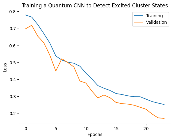
plt.plot(history.history['loss'][1:], label='Training')
plt.plot(history.history['val_loss'][1:], label='Validation')
plt.title('Training a Quantum CNN to Detect Excited Cluster States')
plt.xlabel('Epochs')
plt.ylabel('Loss')
plt.legend()
plt.show()

png

2. Model hibrida

Anda tidak perlu beralih dari delapan qubit ke satu qubit menggunakan konvolusi kuantum—Anda bisa melakukan satu atau dua putaran konvolusi kuantum dan memasukkan hasilnya ke dalam jaringan saraf klasik. Bagian ini mengeksplorasi model hibrida kuantum-klasik.

2.1 Model hibrida dengan filter kuantum tunggal

Terapkan satu lapisan konvolusi kuantum, membacakan \(\langle \hat{Z}_n \rangle\) pada semua bit, diikuti oleh jaringan saraf yang terhubung secara padat.

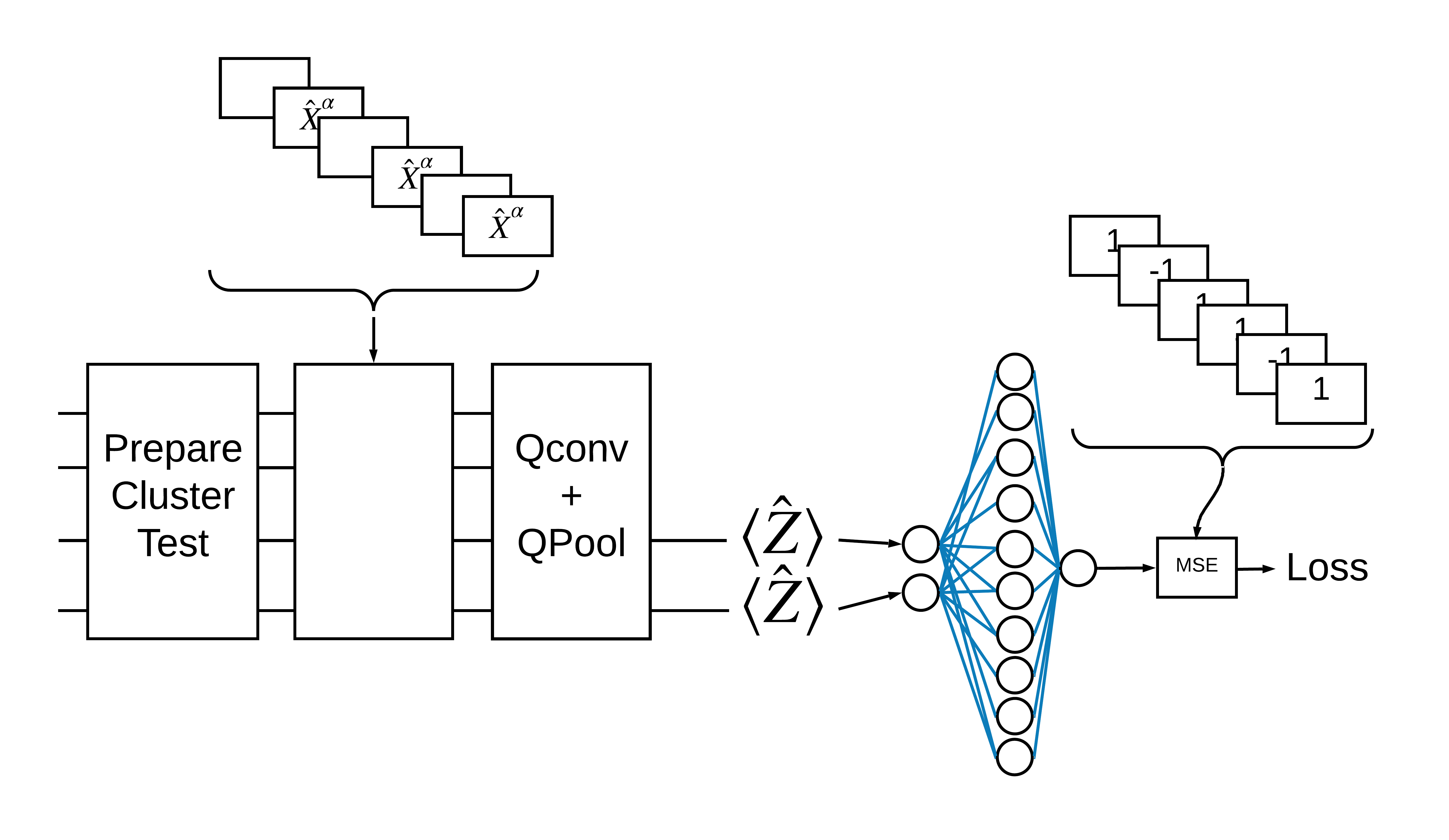
2.1.1 Definisi model

# 1-local operators to read out
readouts = [cirq.Z(bit) for bit in cluster_state_bits[4:]]


def multi_readout_model_circuit(qubits):
    """Make a model circuit with less quantum pool and conv operations."""
    model_circuit = cirq.Circuit()
    symbols = sympy.symbols('qconv0:21')
    model_circuit += quantum_conv_circuit(qubits, symbols[0:15])
    model_circuit += quantum_pool_circuit(qubits[:4], qubits[4:],
                                          symbols[15:21])
    return model_circuit


# Build a model enacting the logic in 2.1 of this notebook.
excitation_input_dual = tf.keras.Input(shape=(), dtype=tf.dtypes.string)

cluster_state_dual = tfq.layers.AddCircuit()(
    excitation_input_dual, prepend=cluster_state_circuit(cluster_state_bits))

quantum_model_dual = tfq.layers.PQC(
    multi_readout_model_circuit(cluster_state_bits),
    readouts)(cluster_state_dual)

d1_dual = tf.keras.layers.Dense(8)(quantum_model_dual)

d2_dual = tf.keras.layers.Dense(1)(d1_dual)

hybrid_model = tf.keras.Model(inputs=[excitation_input_dual], outputs=[d2_dual])

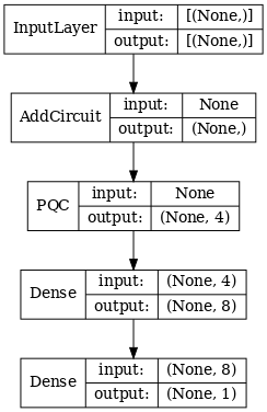
# Display the model architecture
tf.keras.utils.plot_model(hybrid_model,
                          show_shapes=True,
                          show_layer_names=False,
                          dpi=70)

png

2.1.2 Melatih model

hybrid_model.compile(optimizer=tf.keras.optimizers.Adam(learning_rate=0.02),
                     loss=tf.losses.mse,
                     metrics=[custom_accuracy])

hybrid_history = hybrid_model.fit(x=train_excitations,
                                  y=train_labels,
                                  batch_size=16,
                                  epochs=25,
                                  verbose=1,
                                  validation_data=(test_excitations,
                                                   test_labels))

Epoch 1/25
7/7 [==============================] - 1s 113ms/step - loss: 0.9848 - custom_accuracy: 0.5179 - val_loss: 0.9635 - val_custom_accuracy: 0.5417
Epoch 2/25
7/7 [==============================] - 1s 86ms/step - loss: 0.8095 - custom_accuracy: 0.6339 - val_loss: 0.6800 - val_custom_accuracy: 0.7083
Epoch 3/25
7/7 [==============================] - 1s 85ms/step - loss: 0.4045 - custom_accuracy: 0.9375 - val_loss: 0.3342 - val_custom_accuracy: 0.8750
Epoch 4/25
7/7 [==============================] - 1s 86ms/step - loss: 0.2308 - custom_accuracy: 0.9643 - val_loss: 0.2027 - val_custom_accuracy: 0.9792
Epoch 5/25
7/7 [==============================] - 1s 84ms/step - loss: 0.2232 - custom_accuracy: 0.9554 - val_loss: 0.1761 - val_custom_accuracy: 1.0000
Epoch 6/25
7/7 [==============================] - 1s 84ms/step - loss: 0.1760 - custom_accuracy: 0.9821 - val_loss: 0.2541 - val_custom_accuracy: 0.9167
Epoch 7/25
7/7 [==============================] - 1s 85ms/step - loss: 0.1919 - custom_accuracy: 0.9643 - val_loss: 0.1967 - val_custom_accuracy: 0.9792
Epoch 8/25
7/7 [==============================] - 1s 83ms/step - loss: 0.1892 - custom_accuracy: 0.9554 - val_loss: 0.1870 - val_custom_accuracy: 0.9792
Epoch 9/25
7/7 [==============================] - 1s 84ms/step - loss: 0.1777 - custom_accuracy: 0.9911 - val_loss: 0.2208 - val_custom_accuracy: 0.9583
Epoch 10/25
7/7 [==============================] - 1s 83ms/step - loss: 0.1728 - custom_accuracy: 0.9732 - val_loss: 0.2147 - val_custom_accuracy: 0.9583
Epoch 11/25
7/7 [==============================] - 1s 85ms/step - loss: 0.1704 - custom_accuracy: 0.9732 - val_loss: 0.1810 - val_custom_accuracy: 0.9792
Epoch 12/25
7/7 [==============================] - 1s 85ms/step - loss: 0.1739 - custom_accuracy: 0.9732 - val_loss: 0.2038 - val_custom_accuracy: 0.9792
Epoch 13/25
7/7 [==============================] - 1s 81ms/step - loss: 0.1705 - custom_accuracy: 0.9732 - val_loss: 0.1855 - val_custom_accuracy: 0.9792
Epoch 14/25
7/7 [==============================] - 1s 84ms/step - loss: 0.1788 - custom_accuracy: 0.9643 - val_loss: 0.2152 - val_custom_accuracy: 0.9583
Epoch 15/25
7/7 [==============================] - 1s 84ms/step - loss: 0.1760 - custom_accuracy: 0.9732 - val_loss: 0.1994 - val_custom_accuracy: 1.0000
Epoch 16/25
7/7 [==============================] - 1s 83ms/step - loss: 0.1737 - custom_accuracy: 0.9732 - val_loss: 0.2035 - val_custom_accuracy: 0.9792
Epoch 17/25
7/7 [==============================] - 1s 82ms/step - loss: 0.1749 - custom_accuracy: 0.9911 - val_loss: 0.1983 - val_custom_accuracy: 0.9583
Epoch 18/25
7/7 [==============================] - 1s 83ms/step - loss: 0.1875 - custom_accuracy: 0.9732 - val_loss: 0.1916 - val_custom_accuracy: 0.9583
Epoch 19/25
7/7 [==============================] - 1s 82ms/step - loss: 0.1605 - custom_accuracy: 0.9732 - val_loss: 0.1782 - val_custom_accuracy: 0.9792
Epoch 20/25
7/7 [==============================] - 1s 84ms/step - loss: 0.1668 - custom_accuracy: 0.9911 - val_loss: 0.2276 - val_custom_accuracy: 0.9583
Epoch 21/25
7/7 [==============================] - 1s 84ms/step - loss: 0.1700 - custom_accuracy: 0.9911 - val_loss: 0.2080 - val_custom_accuracy: 0.9583
Epoch 22/25
7/7 [==============================] - 1s 83ms/step - loss: 0.1621 - custom_accuracy: 0.9732 - val_loss: 0.1851 - val_custom_accuracy: 0.9375
Epoch 23/25
7/7 [==============================] - 1s 84ms/step - loss: 0.1695 - custom_accuracy: 0.9911 - val_loss: 0.1882 - val_custom_accuracy: 0.9792
Epoch 24/25
7/7 [==============================] - 1s 82ms/step - loss: 0.1583 - custom_accuracy: 0.9911 - val_loss: 0.2017 - val_custom_accuracy: 0.9583
Epoch 25/25
7/7 [==============================] - 1s 83ms/step - loss: 0.1557 - custom_accuracy: 0.9911 - val_loss: 0.1907 - val_custom_accuracy: 0.9792

plt.plot(history.history['val_custom_accuracy'], label='QCNN')
plt.plot(hybrid_history.history['val_custom_accuracy'], label='Hybrid CNN')
plt.title('Quantum vs Hybrid CNN performance')
plt.xlabel('Epochs')
plt.legend()
plt.ylabel('Validation Accuracy')
plt.show()

png

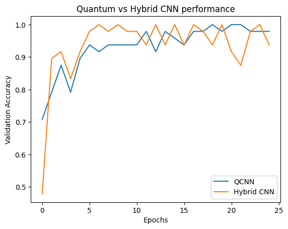
Seperti yang Anda lihat, dengan bantuan klasik yang sangat sederhana, model hibrida biasanya akan menyatu lebih cepat daripada versi kuantum murni.

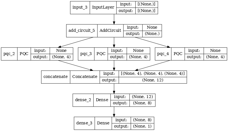
2.2 Konvolusi hibrida dengan beberapa filter kuantum

Sekarang mari kita coba arsitektur yang menggunakan beberapa konvolusi kuantum dan jaringan saraf klasik untuk menggabungkannya.

2.2.1 Definisi model

excitation_input_multi = tf.keras.Input(shape=(), dtype=tf.dtypes.string)

cluster_state_multi = tfq.layers.AddCircuit()(
    excitation_input_multi, prepend=cluster_state_circuit(cluster_state_bits))

# apply 3 different filters and measure expectation values

quantum_model_multi1 = tfq.layers.PQC(
    multi_readout_model_circuit(cluster_state_bits),
    readouts)(cluster_state_multi)

quantum_model_multi2 = tfq.layers.PQC(
    multi_readout_model_circuit(cluster_state_bits),
    readouts)(cluster_state_multi)

quantum_model_multi3 = tfq.layers.PQC(
    multi_readout_model_circuit(cluster_state_bits),
    readouts)(cluster_state_multi)

# concatenate outputs and feed into a small classical NN
concat_out = tf.keras.layers.concatenate(
    [quantum_model_multi1, quantum_model_multi2, quantum_model_multi3])

dense_1 = tf.keras.layers.Dense(8)(concat_out)

dense_2 = tf.keras.layers.Dense(1)(dense_1)

multi_qconv_model = tf.keras.Model(inputs=[excitation_input_multi],
                                   outputs=[dense_2])

# Display the model architecture
tf.keras.utils.plot_model(multi_qconv_model,
                          show_shapes=True,
                          show_layer_names=True,
                          dpi=70)

png

2.2.2 Melatih model

multi_qconv_model.compile(
    optimizer=tf.keras.optimizers.Adam(learning_rate=0.02),
    loss=tf.losses.mse,
    metrics=[custom_accuracy])

multi_qconv_history = multi_qconv_model.fit(x=train_excitations,
                                            y=train_labels,
                                            batch_size=16,
                                            epochs=25,
                                            verbose=1,
                                            validation_data=(test_excitations,
                                                             test_labels))

Epoch 1/25
7/7 [==============================] - 2s 143ms/step - loss: 0.9425 - custom_accuracy: 0.6429 - val_loss: 0.8120 - val_custom_accuracy: 0.7083
Epoch 2/25
7/7 [==============================] - 1s 109ms/step - loss: 0.5778 - custom_accuracy: 0.7946 - val_loss: 0.5920 - val_custom_accuracy: 0.7500
Epoch 3/25
7/7 [==============================] - 1s 103ms/step - loss: 0.4954 - custom_accuracy: 0.9018 - val_loss: 0.4568 - val_custom_accuracy: 0.7708
Epoch 4/25
7/7 [==============================] - 1s 95ms/step - loss: 0.2855 - custom_accuracy: 0.9196 - val_loss: 0.2792 - val_custom_accuracy: 0.9375
Epoch 5/25
7/7 [==============================] - 1s 93ms/step - loss: 0.1902 - custom_accuracy: 0.9821 - val_loss: 0.2212 - val_custom_accuracy: 0.9375
Epoch 6/25
7/7 [==============================] - 1s 94ms/step - loss: 0.1685 - custom_accuracy: 0.9821 - val_loss: 0.2341 - val_custom_accuracy: 0.9583
Epoch 7/25
7/7 [==============================] - 1s 104ms/step - loss: 0.1671 - custom_accuracy: 0.9911 - val_loss: 0.2062 - val_custom_accuracy: 0.9792
Epoch 8/25
7/7 [==============================] - 1s 97ms/step - loss: 0.1511 - custom_accuracy: 0.9821 - val_loss: 0.2096 - val_custom_accuracy: 0.9792
Epoch 9/25
7/7 [==============================] - 1s 96ms/step - loss: 0.1432 - custom_accuracy: 0.9911 - val_loss: 0.2330 - val_custom_accuracy: 0.9375
Epoch 10/25
7/7 [==============================] - 1s 92ms/step - loss: 0.1668 - custom_accuracy: 0.9821 - val_loss: 0.2344 - val_custom_accuracy: 0.9583
Epoch 11/25
7/7 [==============================] - 1s 106ms/step - loss: 0.1893 - custom_accuracy: 0.9732 - val_loss: 0.2148 - val_custom_accuracy: 0.9583
Epoch 12/25
7/7 [==============================] - 1s 104ms/step - loss: 0.1857 - custom_accuracy: 0.9732 - val_loss: 0.2739 - val_custom_accuracy: 0.9583
Epoch 13/25
7/7 [==============================] - 1s 106ms/step - loss: 0.1748 - custom_accuracy: 0.9732 - val_loss: 0.2366 - val_custom_accuracy: 0.9583
Epoch 14/25
7/7 [==============================] - 1s 103ms/step - loss: 0.1515 - custom_accuracy: 0.9821 - val_loss: 0.2012 - val_custom_accuracy: 0.9583
Epoch 15/25
7/7 [==============================] - 1s 100ms/step - loss: 0.1552 - custom_accuracy: 0.9911 - val_loss: 0.2404 - val_custom_accuracy: 0.9375
Epoch 16/25
7/7 [==============================] - 1s 97ms/step - loss: 0.1572 - custom_accuracy: 0.9911 - val_loss: 0.2779 - val_custom_accuracy: 0.9375
Epoch 17/25
7/7 [==============================] - 1s 100ms/step - loss: 0.1546 - custom_accuracy: 0.9821 - val_loss: 0.2104 - val_custom_accuracy: 0.9583
Epoch 18/25
7/7 [==============================] - 1s 102ms/step - loss: 0.1418 - custom_accuracy: 0.9911 - val_loss: 0.2647 - val_custom_accuracy: 0.9583
Epoch 19/25
7/7 [==============================] - 1s 98ms/step - loss: 0.1590 - custom_accuracy: 0.9732 - val_loss: 0.2154 - val_custom_accuracy: 0.9583
Epoch 20/25
7/7 [==============================] - 1s 104ms/step - loss: 0.1363 - custom_accuracy: 1.0000 - val_loss: 0.2470 - val_custom_accuracy: 0.9375
Epoch 21/25
7/7 [==============================] - 1s 100ms/step - loss: 0.1442 - custom_accuracy: 0.9821 - val_loss: 0.2383 - val_custom_accuracy: 0.9375
Epoch 22/25
7/7 [==============================] - 1s 99ms/step - loss: 0.1415 - custom_accuracy: 0.9911 - val_loss: 0.2324 - val_custom_accuracy: 0.9583
Epoch 23/25
7/7 [==============================] - 1s 97ms/step - loss: 0.1424 - custom_accuracy: 0.9821 - val_loss: 0.2188 - val_custom_accuracy: 0.9583
Epoch 24/25
7/7 [==============================] - 1s 100ms/step - loss: 0.1417 - custom_accuracy: 0.9821 - val_loss: 0.2340 - val_custom_accuracy: 0.9375
Epoch 25/25
7/7 [==============================] - 1s 103ms/step - loss: 0.1471 - custom_accuracy: 0.9732 - val_loss: 0.2252 - val_custom_accuracy: 0.9583

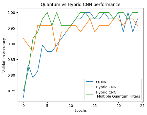
plt.plot(history.history['val_custom_accuracy'][:25], label='QCNN')
plt.plot(hybrid_history.history['val_custom_accuracy'][:25], label='Hybrid CNN')
plt.plot(multi_qconv_history.history['val_custom_accuracy'][:25],
         label='Hybrid CNN \n Multiple Quantum Filters')
plt.title('Quantum vs Hybrid CNN performance')
plt.xlabel('Epochs')
plt.legend()
plt.ylabel('Validation Accuracy')
plt.show()

png