
| |
|
 GitHubでソースを表示 GitHubでソースを表示 |
このチュートリアルでは、WAV 形式の音声ファイルを前処理し、基本的な自動音声認識 (ASR) モデルを構築およびトレーニングして 10 の異なる単語を認識させる方法を示します。Speech Commands データセット (Warden, 2018) の一部を使用します。これには、「down」、「go」、「left」、「no」、「right」、「stop」、「up」、「yes」などのコマンドの短い (1 秒以下) 音声クリップが含まれています。
現実世界の音声認識システムは複雑ですが、MNIST データセットを使用した画像分類と同様に、このチュートリアルでは、関連する基本的な手法について説明します。
セットアップ
必要なモジュールと依存関係をインポートします。ここでは、.wav ファイルから音声分類データセットを生成する際に役立つ tf.keras.utils.audio_dataset_from_directory(TensorFlow 2.10 で導入)を使用します。このチュートリアルでは、可視化を行うための seaborn も必要です。
pip install -U -q tensorflow tensorflow_datasetsimport os
import pathlib
import matplotlib.pyplot as plt
import numpy as np
import seaborn as sns
import tensorflow as tf
from tensorflow.keras import layers
from tensorflow.keras import models
from IPython import display
# Set the seed value for experiment reproducibility.
seed = 42
tf.random.set_seed(seed)
np.random.seed(seed)
2024-01-11 22:07:31.258054: E external/local_xla/xla/stream_executor/cuda/cuda_dnn.cc:9261] Unable to register cuDNN factory: Attempting to register factory for plugin cuDNN when one has already been registered
2024-01-11 22:07:31.258099: E external/local_xla/xla/stream_executor/cuda/cuda_fft.cc:607] Unable to register cuFFT factory: Attempting to register factory for plugin cuFFT when one has already been registered
2024-01-11 22:07:31.259707: E external/local_xla/xla/stream_executor/cuda/cuda_blas.cc:1515] Unable to register cuBLAS factory: Attempting to register factory for plugin cuBLAS when one has already been registered
Mini Speech Commands データセットをインポートする
データの読み込みにかかる時間を短縮するために、Speech Commands データセットの小さいバージョンを使用します。元のデータセットには、105,000 を超える WAV (波形) ファイル形式の音声ファイルが含まれており、様々な人が 35 個の英単語を発音しています。このデータは Google によって収集され、CC BY ライセンスの下で公開されました。
tf.keras.utils.get_file を使用して、小さな音声コマンドデータセットを含む mini_speech_commands.zip ファイルをダウンロードして解凍します。
DATASET_PATH = 'data/mini_speech_commands'

data_dir = pathlib.Path(DATASET_PATH)
if not data_dir.exists():
  tf.keras.utils.get_file(
      'mini_speech_commands.zip',
      origin="http://storage.googleapis.com/download.tensorflow.org/data/mini_speech_commands.zip",
      extract=True,
      cache_dir='.', cache_subdir='data')
Downloading data from http://storage.googleapis.com/download.tensorflow.org/data/mini_speech_commands.zip
182082353/182082353 [==============================] - 1s 0us/step
データセットの音声クリップは、各音声コマンド (no、yes、down、go、left、up、right、stop) に対応する 8 つのフォルダに保存されています。
commands = np.array(tf.io.gfile.listdir(str(data_dir)))
commands = commands[(commands != 'README.md') & (commands != '.DS_Store')]
print('Commands:', commands)
Commands: ['down' 'stop' 'right' 'yes' 'up' 'go' 'left' 'no']
このようにディレクトリに分割すると、keras.utils.audio_dataset_from_directory を使用してデータを簡単に読み込めます。
音声クリップは 16kHz で 1 秒以下です。 output_sequence_length=16000 は、簡単にバッチ処理できるように、短いものを正確に 1 秒にパディングします (長いものはトリミングします)。
train_ds, val_ds = tf.keras.utils.audio_dataset_from_directory(
    directory=data_dir,
    batch_size=64,
    validation_split=0.2,
    seed=0,
    output_sequence_length=16000,
    subset='both')

label_names = np.array(train_ds.class_names)
print()
print("label names:", label_names)
Found 8000 files belonging to 8 classes.
Using 6400 files for training.
Using 1600 files for validation.

label names: ['down' 'go' 'left' 'no' 'right' 'stop' 'up' 'yes']
データセットには、音声クリップと整数ラベルのバッチが含まれるようになりました。音声クリップの形状は (batch, samples, channels) です。
train_ds.element_spec
(TensorSpec(shape=(None, 16000, None), dtype=tf.float32, name=None),
 TensorSpec(shape=(None,), dtype=tf.int32, name=None))
このデータセットには単一チャンネルの音声しか含まれていないため、tf.squeeze 関数を使用して余分な軸を削除します。
def squeeze(audio, labels):
  audio = tf.squeeze(audio, axis=-1)
  return audio, labels

train_ds = train_ds.map(squeeze, tf.data.AUTOTUNE)
val_ds = val_ds.map(squeeze, tf.data.AUTOTUNE)
utils.audio_dataset_from_directory 関数は、最大 2 つの分割のみを返します。テストセットを検証セットとは別にしておくことをお勧めします。別のディレクトリに保存するのが理想的ですが、この場合は Dataset.shard を使用して検証セットを 2 つに分割できます。任意のシャードを反復処理すると、すべてのデータが読み込まれ、その一部のみが保持されることに注意してください。
test_ds = val_ds.shard(num_shards=2, index=0)
val_ds = val_ds.shard(num_shards=2, index=1)
for example_audio, example_labels in train_ds.take(1):
  print(example_audio.shape)
  print(example_labels.shape)
(64, 16000)
(64,)
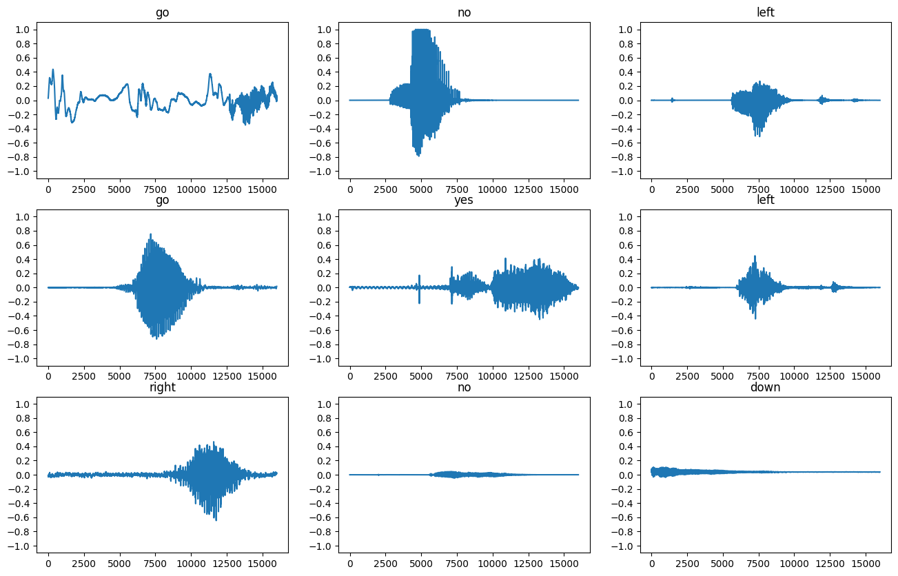
いくつかの音声波形をプロットします。
label_names[[1,1,3,0]]
array(['go', 'go', 'no', 'down'], dtype='<U5')
plt.figure(figsize=(16, 10))
rows = 3
cols = 3
n = rows * cols
for i in range(n):
  plt.subplot(rows, cols, i+1)
  audio_signal = example_audio[i]
  plt.plot(audio_signal)
  plt.title(label_names[example_labels[i]])
  plt.yticks(np.arange(-1.2, 1.2, 0.2))
  plt.ylim([-1.1, 1.1])
波形をスペクトログラムに変換
データセットの波形は時間ドメインで表されます。次に、短時間フーリエ変換 (STFT) を計算して波形をスペクトログラムに変換することにより、波形を時間ドメイン信号から時間周波数ドメイン信号に変換します。時間の経過に伴う周波の変化を示し、2D 画像として表すことができます。スペクトログラム画像をニューラル ネットワークにフィードして、モデルをトレーニングします。
フーリエ変換 (tf.signal.fft) は、信号をその成分の周波数に変換しますが、すべての時間情報は失われます。対照的に、STFT (tf.signal.stft) は信号を時間のウィンドウに分割し、時間情報を保持して各ウィンドウでフーリエ変換を実行し、2D テンソルを返すので標準の畳み込みを実行できます。
波形をスペクトログラムに変換するユーティリティ関数を作成します。
- 波形をスペクトログラムに変換する場合、結果が同様の次元になるように、波形は同じ長さである必要があります。そのために、1 秒未満の音声クリップはゼロパディングします (
tf.zerosを使用)。 tf.signal.stftを呼び出すときは、生成されたスペクトログラム「画像」がほぼ正方形になるようにframe_lengthおよびframe_stepパラメータを選択します。STFT パラメータの選択の詳細については、音声信号処理と STFT に関するこの Coursera 動画を参照してください。- STFT は、大きさと位相を表す複素数の配列を生成します。ただし、このチュートリアルでは、
tf.signal.stftの出力にtf.absを適用することで導出できる大きさのみを使用します。
def get_spectrogram(waveform):
  # Convert the waveform to a spectrogram via a STFT.
  spectrogram = tf.signal.stft(
      waveform, frame_length=255, frame_step=128)
  # Obtain the magnitude of the STFT.
  spectrogram = tf.abs(spectrogram)
  # Add a `channels` dimension, so that the spectrogram can be used
  # as image-like input data with convolution layers (which expect
  # shape (`batch_size`, `height`, `width`, `channels`).
  spectrogram = spectrogram[..., tf.newaxis]
  return spectrogram
次に、データを探索します。1 つの例のテンソル化された波形と対応するスペクトログラムの形状を出力し、元の音声を再生します。
for i in range(3):
  label = label_names[example_labels[i]]
  waveform = example_audio[i]
  spectrogram = get_spectrogram(waveform)

  print('Label:', label)
  print('Waveform shape:', waveform.shape)
  print('Spectrogram shape:', spectrogram.shape)
  print('Audio playback')
  display.display(display.Audio(waveform, rate=16000))
Label: go
Waveform shape: (16000,)
Spectrogram shape: (124, 129, 1)
Audio playback
Label: no
Waveform shape: (16000,)
Spectrogram shape: (124, 129, 1)
Audio playback
Label: left
Waveform shape: (16000,)
Spectrogram shape: (124, 129, 1)
Audio playback
次に、スペクトログラムを表示する関数を定義します。
def plot_spectrogram(spectrogram, ax):
  if len(spectrogram.shape) > 2:
    assert len(spectrogram.shape) == 3
    spectrogram = np.squeeze(spectrogram, axis=-1)
  # Convert the frequencies to log scale and transpose, so that the time is
  # represented on the x-axis (columns).
  # Add an epsilon to avoid taking a log of zero.
  log_spec = np.log(spectrogram.T + np.finfo(float).eps)
  height = log_spec.shape[0]
  width = log_spec.shape[1]
  X = np.linspace(0, np.size(spectrogram), num=width, dtype=int)
  Y = range(height)
  ax.pcolormesh(X, Y, log_spec)
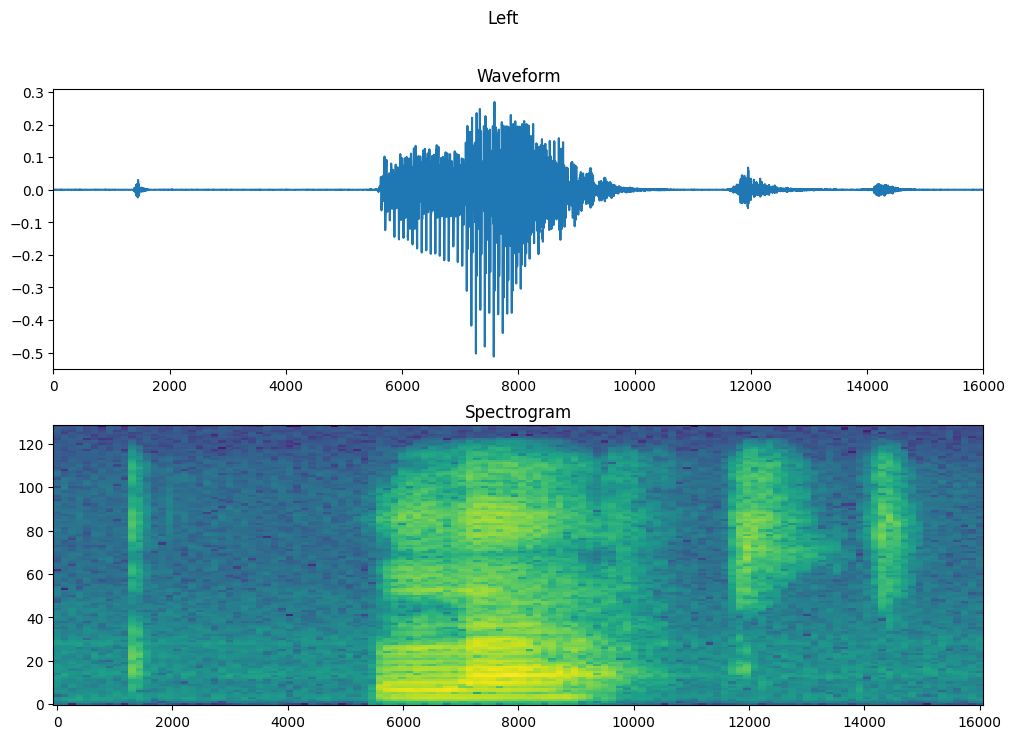
時間の経過に伴う例の波形と、対応するスペクトログラム (時間の経過に伴う周波数) をプロットします。
fig, axes = plt.subplots(2, figsize=(12, 8))
timescale = np.arange(waveform.shape[0])
axes[0].plot(timescale, waveform.numpy())
axes[0].set_title('Waveform')
axes[0].set_xlim([0, 16000])

plot_spectrogram(spectrogram.numpy(), axes[1])
axes[1].set_title('Spectrogram')
plt.suptitle(label.title())
plt.show()
音声データセットからスペクトログラムデータセットを作成します。
def make_spec_ds(ds):
  return ds.map(
      map_func=lambda audio,label: (get_spectrogram(audio), label),
      num_parallel_calls=tf.data.AUTOTUNE)
train_spectrogram_ds = make_spec_ds(train_ds)
val_spectrogram_ds = make_spec_ds(val_ds)
test_spectrogram_ds = make_spec_ds(test_ds)
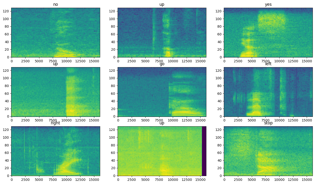
データセットのさまざまな例のスペクトログラムを調べます。
for example_spectrograms, example_spect_labels in train_spectrogram_ds.take(1):
  break
rows = 3
cols = 3
n = rows*cols
fig, axes = plt.subplots(rows, cols, figsize=(16, 9))

for i in range(n):
    r = i // cols
    c = i % cols
    ax = axes[r][c]
    plot_spectrogram(example_spectrograms[i].numpy(), ax)
    ax.set_title(label_names[example_spect_labels[i].numpy()])

plt.show()
モデルを構築してトレーニングする
Dataset.cache と Dataset.prefetch 演算を追加して、モデルのトレーニング時の読み取りレイテンシを短縮します。
train_spectrogram_ds = train_spectrogram_ds.cache().shuffle(10000).prefetch(tf.data.AUTOTUNE)
val_spectrogram_ds = val_spectrogram_ds.cache().prefetch(tf.data.AUTOTUNE)
test_spectrogram_ds = test_spectrogram_ds.cache().prefetch(tf.data.AUTOTUNE)
音声ファイルをスペクトログラム画像に変換したので、モデルで単純な畳み込みニューラル ネットワーク (CNN) を使用します。
tf.keras.Sequential モデルは、次の Keras 前処理レイヤーを使用します。
tf.keras.layers.Resizingは入力をダウンサンプリングし、モデルをより迅速にトレーニングできるようにします。tf.keras.layers.Normalizationは平均値と標準偏差に基づいて画像内の各ピクセルを正規化します。
Normalization レイヤーの場合、まずトレーニングデータに対して adapt メソッドを呼び出して、集計統計 (平均と標準偏差) を計算する必要があります。
input_shape = example_spectrograms.shape[1:]
print('Input shape:', input_shape)
num_labels = len(label_names)

# Instantiate the `tf.keras.layers.Normalization` layer.
norm_layer = layers.Normalization()
# Fit the state of the layer to the spectrograms
# with `Normalization.adapt`.
norm_layer.adapt(data=train_spectrogram_ds.map(map_func=lambda spec, label: spec))

model = models.Sequential([
    layers.Input(shape=input_shape),
    # Downsample the input.
    layers.Resizing(32, 32),
    # Normalize.
    norm_layer,
    layers.Conv2D(32, 3, activation='relu'),
    layers.Conv2D(64, 3, activation='relu'),
    layers.MaxPooling2D(),
    layers.Dropout(0.25),
    layers.Flatten(),
    layers.Dense(128, activation='relu'),
    layers.Dropout(0.5),
    layers.Dense(num_labels),
])

model.summary()
Input shape: (124, 129, 1)
Model: "sequential"
_________________________________________________________________
 Layer (type)                Output Shape              Param #
=================================================================
 resizing (Resizing)         (None, 32, 32, 1)         0

 normalization (Normalizati  (None, 32, 32, 1)         3
 on)

 conv2d (Conv2D)             (None, 30, 30, 32)        320

 conv2d_1 (Conv2D)           (None, 28, 28, 64)        18496

 max_pooling2d (MaxPooling2  (None, 14, 14, 64)        0
 D)

 dropout (Dropout)           (None, 14, 14, 64)        0

 flatten (Flatten)           (None, 12544)             0

 dense (Dense)               (None, 128)               1605760

 dropout_1 (Dropout)         (None, 128)               0

 dense_1 (Dense)             (None, 8)                 1032

=================================================================
Total params: 1625611 (6.20 MB)
Trainable params: 1625608 (6.20 MB)
Non-trainable params: 3 (16.00 Byte)
_________________________________________________________________
Adam オプティマイザとクロスエントロピー損失を使用して Keras モデルを構成します。
model.compile(
    optimizer=tf.keras.optimizers.Adam(),
    loss=tf.keras.losses.SparseCategoricalCrossentropy(from_logits=True),
    metrics=['accuracy'],
)
デモするために、モデルを 10 エポックにわたってトレーニングします。
EPOCHS = 10
history = model.fit(
    train_spectrogram_ds,
    validation_data=val_spectrogram_ds,
    epochs=EPOCHS,
    callbacks=tf.keras.callbacks.EarlyStopping(verbose=1, patience=2),
)
Epoch 1/10
2024-01-11 22:07:47.222482: E tensorflow/core/grappler/optimizers/meta_optimizer.cc:961] layout failed: INVALID_ARGUMENT: Size of values 0 does not match size of permutation 4 @ fanin shape insequential/dropout/dropout/SelectV2-2-TransposeNHWCToNCHW-LayoutOptimizer
WARNING: All log messages before absl::InitializeLog() is called are written to STDERR
I0000 00:00:1705010869.111571 1000761 device_compiler.h:186] Compiled cluster using XLA!  This line is logged at most once for the lifetime of the process.
100/100 [==============================] - 5s 12ms/step - loss: 1.7746 - accuracy: 0.3548 - val_loss: 1.3972 - val_accuracy: 0.5586
Epoch 2/10
100/100 [==============================] - 1s 8ms/step - loss: 1.2599 - accuracy: 0.5605 - val_loss: 0.9920 - val_accuracy: 0.6927
Epoch 3/10
100/100 [==============================] - 1s 8ms/step - loss: 0.9657 - accuracy: 0.6648 - val_loss: 0.8118 - val_accuracy: 0.7591
Epoch 4/10
100/100 [==============================] - 1s 8ms/step - loss: 0.7856 - accuracy: 0.7223 - val_loss: 0.6963 - val_accuracy: 0.7812
Epoch 5/10
100/100 [==============================] - 1s 8ms/step - loss: 0.6674 - accuracy: 0.7680 - val_loss: 0.6225 - val_accuracy: 0.8164
Epoch 6/10
100/100 [==============================] - 1s 8ms/step - loss: 0.5725 - accuracy: 0.7986 - val_loss: 0.6141 - val_accuracy: 0.7917
Epoch 7/10
100/100 [==============================] - 1s 8ms/step - loss: 0.5319 - accuracy: 0.8112 - val_loss: 0.5328 - val_accuracy: 0.8307
Epoch 8/10
100/100 [==============================] - 1s 8ms/step - loss: 0.4793 - accuracy: 0.8336 - val_loss: 0.5316 - val_accuracy: 0.8346
Epoch 9/10
100/100 [==============================] - 1s 8ms/step - loss: 0.4262 - accuracy: 0.8466 - val_loss: 0.4979 - val_accuracy: 0.8294
Epoch 10/10
100/100 [==============================] - 1s 8ms/step - loss: 0.3870 - accuracy: 0.8623 - val_loss: 0.4751 - val_accuracy: 0.8385
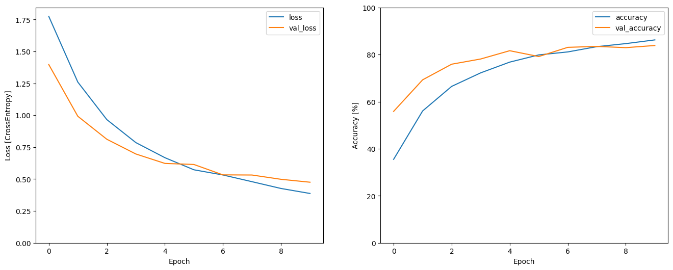
トレーニングと検証の損失曲線をプロットして、トレーニング中にモデルがどのように改善されたかを確認します。
metrics = history.history
plt.figure(figsize=(16,6))
plt.subplot(1,2,1)
plt.plot(history.epoch, metrics['loss'], metrics['val_loss'])
plt.legend(['loss', 'val_loss'])
plt.ylim([0, max(plt.ylim())])
plt.xlabel('Epoch')
plt.ylabel('Loss [CrossEntropy]')

plt.subplot(1,2,2)
plt.plot(history.epoch, 100*np.array(metrics['accuracy']), 100*np.array(metrics['val_accuracy']))
plt.legend(['accuracy', 'val_accuracy'])
plt.ylim([0, 100])
plt.xlabel('Epoch')
plt.ylabel('Accuracy [%]')
Text(0, 0.5, 'Accuracy [%]')
モデルのパフォーマンスを評価する
テストセットでモデルを実行し、モデルのパフォーマンスを確認します。
model.evaluate(test_spectrogram_ds, return_dict=True)
13/13 [==============================] - 0s 6ms/step - loss: 0.4939 - accuracy: 0.8329
{'loss': 0.49389326572418213, 'accuracy': 0.832932710647583}
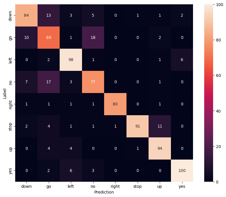
混同行列を表示する
混同行列を使用して、モデルがテストセット内の各コマンドをどの程度うまく分類したかを確認します。
y_pred = model.predict(test_spectrogram_ds)
13/13 [==============================] - 0s 3ms/step
y_pred = tf.argmax(y_pred, axis=1)
y_true = tf.concat(list(test_spectrogram_ds.map(lambda s,lab: lab)), axis=0)
confusion_mtx = tf.math.confusion_matrix(y_true, y_pred)
plt.figure(figsize=(10, 8))
sns.heatmap(confusion_mtx,
            xticklabels=label_names,
            yticklabels=label_names,
            annot=True, fmt='g')
plt.xlabel('Prediction')
plt.ylabel('Label')
plt.show()
音声ファイルで推論を実行する
最後に、誰かが「no」と言っている入力音声ファイルを使用して、モデルの予測出力を検証します。モデルのパフォーマンスはどうですか?
x = data_dir/'no/01bb6a2a_nohash_0.wav'
x = tf.io.read_file(str(x))
x, sample_rate = tf.audio.decode_wav(x, desired_channels=1, desired_samples=16000,)
x = tf.squeeze(x, axis=-1)
waveform = x
x = get_spectrogram(x)
x = x[tf.newaxis,...]

prediction = model(x)
x_labels = ['no', 'yes', 'down', 'go', 'left', 'up', 'right', 'stop']
plt.bar(x_labels, tf.nn.softmax(prediction[0]))
plt.title('No')
plt.show()

display.display(display.Audio(waveform, rate=16000))
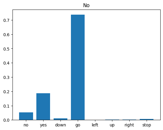
出力が示すように、モデルは音声コマンドを「no」として認識しているはずです。
モデルを前処理してエクスポートする
推論のためにデータをモデルに渡す前に、これらの前処理手順を適用する必要がある場合、このモデルはあまり簡単に使用できません。そのため、エンドツーエンドのバージョンをビルドします。
class ExportModel(tf.Module):
  def __init__(self, model):
    self.model = model

    # Accept either a string-filename or a batch of waveforms.
    # YOu could add additional signatures for a single wave, or a ragged-batch.
    self.__call__.get_concrete_function(
        x=tf.TensorSpec(shape=(), dtype=tf.string))
    self.__call__.get_concrete_function(
       x=tf.TensorSpec(shape=[None, 16000], dtype=tf.float32))


  @tf.function
  def __call__(self, x):
    # If they pass a string, load the file and decode it.
    if x.dtype == tf.string:
      x = tf.io.read_file(x)
      x, _ = tf.audio.decode_wav(x, desired_channels=1, desired_samples=16000,)
      x = tf.squeeze(x, axis=-1)
      x = x[tf.newaxis, :]

    x = get_spectrogram(x)
    result = self.model(x, training=False)

    class_ids = tf.argmax(result, axis=-1)
    class_names = tf.gather(label_names, class_ids)
    return {'predictions':result,
            'class_ids': class_ids,
            'class_names': class_names}
「エクスポート」モデルをテスト実行します。
export = ExportModel(model)
export(tf.constant(str(data_dir/'no/01bb6a2a_nohash_0.wav')))
{'predictions': <tf.Tensor: shape=(1, 8), dtype=float32, numpy=
 array([[ 0.57496786,  1.8535713 , -0.936327  ,  3.2253902 , -4.3184023 ,
         -2.7080545 , -2.3667598 , -1.3555104 ]], dtype=float32)>,
 'class_ids': <tf.Tensor: shape=(1,), dtype=int64, numpy=array([3])>,
 'class_names': <tf.Tensor: shape=(1,), dtype=string, numpy=array([b'no'], dtype=object)>}
モデルを保存して再読み込みすると、再読み込みされたモデルから同じ出力が得られます。
tf.saved_model.save(export, "saved")
imported = tf.saved_model.load("saved")
imported(waveform[tf.newaxis, :])
INFO:tensorflow:Assets written to: saved/assets
INFO:tensorflow:Assets written to: saved/assets
{'class_names': <tf.Tensor: shape=(1,), dtype=string, numpy=array([b'no'], dtype=object)>,
 'predictions': <tf.Tensor: shape=(1, 8), dtype=float32, numpy=
 array([[ 0.57496786,  1.8535713 , -0.936327  ,  3.2253902 , -4.3184023 ,
         -2.7080545 , -2.3667598 , -1.3555104 ]], dtype=float32)>,
 'class_ids': <tf.Tensor: shape=(1,), dtype=int64, numpy=array([3])>}
次のステップ
このチュートリアルでは、TensorFlow と Python を使用した畳み込みニューラル ネットワークを使用して、簡単な音声分類/自動音声認識を実行する方法を実演しました。詳細については、次のリソースを参照してください。
- YAMNet による音声分類のチュートリアルでは、音声分類に転移学習を使用する方法を実演します。
- Kaggle の TensorFlow 音声認識チャレンジのノートブック。
- TensorFlow.js - 転移学習コードラボを使用した音声認識では、音声分類用の独自のインタラクティブな Web アプリを構築する方法について説明します。
- 音楽情報検索のためのディープラーニングに関するチュートリアル (Choi et al., 2017)、arXiv。
- また、TensorFlow には、独自の音声ベースのプロジェクトに役立つ音声データの準備と拡張のための追加サポートがあります。
- 音楽および音声分析用の librosa ライブラリの使用を検討してください。