
| |
|
 GitHub에서 소그 보기 GitHub에서 소그 보기 |
이 튜토리얼에서는 Ian Goodfellow et al의 Explaining and Harnessing Adversarial Examples에 기술된 FGSM(Fast Gradient Signed Method)을 이용해 적대적 샘플(adversarial example)을 생성하는 방법에 대해 소개합니다. FGSM은 신경망 공격 기술들 중 초기에 발견된 방법이자 가장 유명한 방식 중 하나입니다.
적대적 샘플이란?
적대적 샘플이란 신경망을 혼란시킬 목적으로 만들어진 특수한 입력으로, 신경망으로 하여금 샘플을 잘못 분류하도록 합니다. 비록 인간에게 적대적 샘플은 일반 샘플과 큰 차이가 없어보이지만, 신경망은 적대적 샘플을 올바르게 식별하지 못합니다. 이와 같은 신경망 공격에는 여러 종류가 있는데, 본 튜토리얼에서는 화이트 박스(white box) 공격 기술에 속하는 FGSM을 소개합니다. 화이트 박스 공격이란 공격자가 대상 모델의 모든 파라미터값에 접근할 수 있다는 가정 하에 이루어지는 공격을 일컫습니다. 아래 이미지는 Goodfellow et al에 소개된 가장 유명한 적대적 샘플인 판다의 사진입니다.
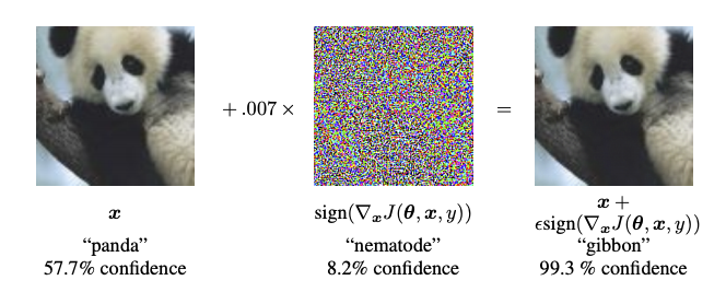
원본 이미지에 특정한 작은 왜곡을 추가하면 신경망으로 하여금 판다를 높은 신뢰도로 긴팔 원숭이로 잘못 인식하도록 만들 수 있습니다. 이하 섹션에서는 이 왜곡 추가 과정에 대해 살펴보도록 하겠습니다.
FGSM
FGSM은 신경망의 그래디언트(gradient)를 이용해 적대적 샘플을 생성하는 기법입니다. 만약 모델의 입력이 이미지라면, 입력 이미지에 대한 손실 함수의 그래디언트를 계산하여 그 손실을 최대화하는 이미지를 생성합니다. 이처럼 새롭게 생성된 이미지를 적대적 이미지(adversarial image)라고 합니다. 이 과정은 다음과 같은 수식으로 정리할 수 있습니다:
\[adv_x = x + \epsilon*\text{sign}(\nabla_xJ(\theta, x, y))\]
- adv_x : 적대적 이미지.
- x : 원본 입력 이미지.
- y : 원본 입력 레이블(label).
- \(\epsilon\) : 왜곡의 양을 적게 만들기 위해 곱하는 수.
- \(\theta\) : 모델의 파라미터.
- \(J\) : 손실 함수.
각 기호에 대한 설명은 다음과 같습니다.
여기서 흥미로운 사실은 입력 이미지에 대한 그래디언트가 사용된다는 점입니다. 이는 손실을 최대화하는 이미지를 생성하는 것이 FGSM의 목적이기 때문입니다. 요약하자면, 적대적 샘플은 각 픽셀의 손실에 대한 기여도를 그래디언트를 통해 계산한 후, 그 기여도에 따라 픽셀값에 왜곡을 추가함으로써 생성할 수 있습니다. 각 픽셀의 기여도는 연쇄 법칙(chain rule)을 이용해 그래디언트를 계산하는 것으로 빠르게 파악할 수 있습니다. 이것이 입력 이미지에 대한 그래디언트가 쓰이는 이유입니다. 또한, 대상 모델은 더 이상 학습하고 있지 않기 때문에 (따라서 신경망의 가중치에 대한 그래디언트는 필요하지 않습니다) 모델의 가중치값은 변하지 않습니다. FGSM의 궁극적인 목표는 이미 학습을 마친 상태의 모델을 혼란시키는 것입니다.
import tensorflow as tf
import matplotlib as mpl
import matplotlib.pyplot as plt

mpl.rcParams['figure.figsize'] = (8, 8)
mpl.rcParams['axes.grid'] = False
2022-12-14 23:32:39.359963: W tensorflow/compiler/xla/stream_executor/platform/default/dso_loader.cc:64] Could not load dynamic library 'libnvinfer.so.7'; dlerror: libnvinfer.so.7: cannot open shared object file: No such file or directory
2022-12-14 23:32:39.360084: W tensorflow/compiler/xla/stream_executor/platform/default/dso_loader.cc:64] Could not load dynamic library 'libnvinfer_plugin.so.7'; dlerror: libnvinfer_plugin.so.7: cannot open shared object file: No such file or directory
2022-12-14 23:32:39.360094: W tensorflow/compiler/tf2tensorrt/utils/py_utils.cc:38] TF-TRT Warning: Cannot dlopen some TensorRT libraries. If you would like to use Nvidia GPU with TensorRT, please make sure the missing libraries mentioned above are installed properly.
사전 훈련된 MobileNetV2 모델과 ImageNet의 클래스(class) 이름들을 불러옵니다.
pretrained_model = tf.keras.applications.MobileNetV2(include_top=True,
                                                     weights='imagenet')
pretrained_model.trainable = False

# ImageNet labels
decode_predictions = tf.keras.applications.mobilenet_v2.decode_predictions
Downloading data from https://storage.googleapis.com/tensorflow/keras-applications/mobilenet_v2/mobilenet_v2_weights_tf_dim_ordering_tf_kernels_1.0_224.h5
14536120/14536120 [==============================] - 0s 0us/step
# Helper function to preprocess the image so that it can be inputted in MobileNetV2
def preprocess(image):
  image = tf.cast(image, tf.float32)
  image = tf.image.resize(image, (224, 224))
  image = tf.keras.applications.mobilenet_v2.preprocess_input(image)
  image = image[None, ...]
  return image

# Helper function to extract labels from probability vector
def get_imagenet_label(probs):
  return decode_predictions(probs, top=1)[0][0]
원본 이미지
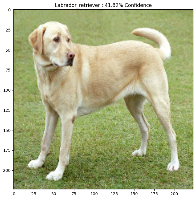
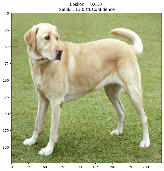
Mirko CC-BY-SA 3.0의 래브라도 리트리버 샘플 이미지를 이용해 적대적 샘플을 생성합니다. 첫 단계로, 원본 이미지를 전처리하여 MobileNetV2 모델에 입력으로 제공합니다.
image_path = tf.keras.utils.get_file('YellowLabradorLooking_new.jpg', 'https://storage.googleapis.com/download.tensorflow.org/example_images/YellowLabradorLooking_new.jpg')
image_raw = tf.io.read_file(image_path)
image = tf.image.decode_image(image_raw)

image = preprocess(image)
image_probs = pretrained_model.predict(image)
Downloading data from https://storage.googleapis.com/download.tensorflow.org/example_images/YellowLabradorLooking_new.jpg
83281/83281 [==============================] - 0s 0us/step
1/1 [==============================] - 2s 2s/step
이미지를 살펴봅시다.
plt.figure()
plt.imshow(image[0] * 0.5 + 0.5)  # To change [-1, 1] to [0,1]
_, image_class, class_confidence = get_imagenet_label(image_probs)
plt.title('{} : {:.2f}% Confidence'.format(image_class, class_confidence*100))
plt.show()
Downloading data from https://storage.googleapis.com/download.tensorflow.org/data/imagenet_class_index.json
35363/35363 [==============================] - 0s 0us/step
적대적 이미지 생성하기
FGSM 실행하기
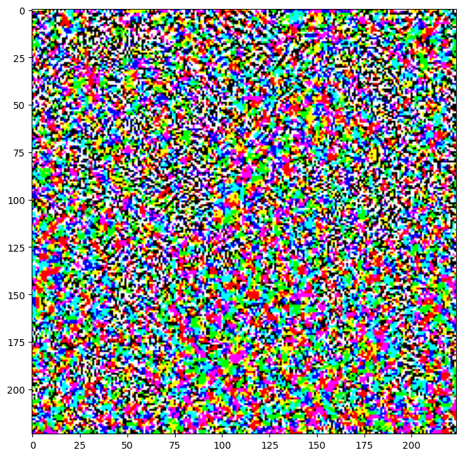
첫번째 단계는 샘플 생성을 위해 원본 이미지에 가하게 될 왜곡을 생성하는 것입니다. 앞서 살펴보았듯이, 왜곡을 생성할 때에는 입력 이미지에 대한 그래디언트를 사용합니다.
loss_object = tf.keras.losses.CategoricalCrossentropy()

def create_adversarial_pattern(input_image, input_label):
  with tf.GradientTape() as tape:
    tape.watch(input_image)
    prediction = pretrained_model(input_image)
    loss = loss_object(input_label, prediction)

  # Get the gradients of the loss w.r.t to the input image.
  gradient = tape.gradient(loss, input_image)
  # Get the sign of the gradients to create the perturbation
  signed_grad = tf.sign(gradient)
  return signed_grad
생성한 왜곡을 시각화해 볼 수 있습니다.
# Get the input label of the image.
labrador_retriever_index = 208
label = tf.one_hot(labrador_retriever_index, image_probs.shape[-1])
label = tf.reshape(label, (1, image_probs.shape[-1]))

perturbations = create_adversarial_pattern(image, label)
plt.imshow(perturbations[0] * 0.5 + 0.5);  # To change [-1, 1] to [0,1]
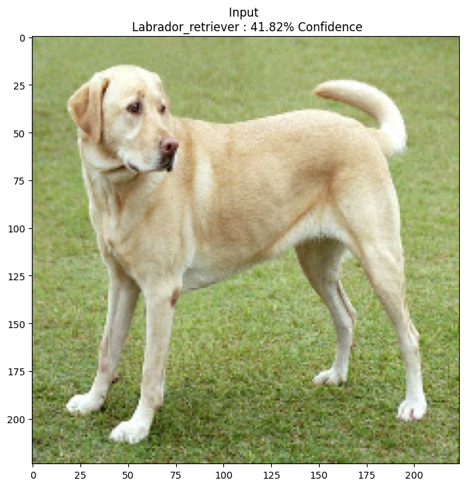
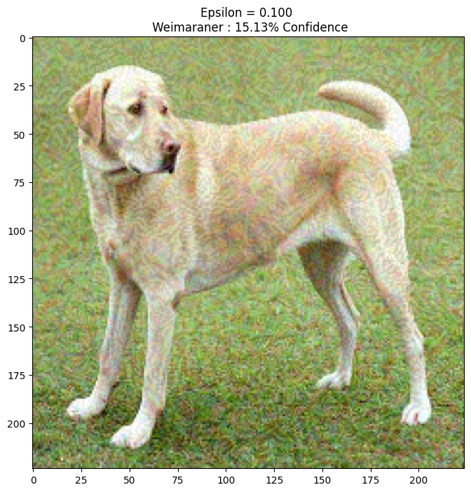
왜곡 승수 엡실론(epsilon)을 바꿔가며 다양한 값들을 시도해봅시다. 위의 간단한 실험을 통해 엡실론의 값이 커질수록 네트워크를 혼란시키는 것이 쉬워짐을 알 수 있습니다. 하지만 이는 이미지의 왜곡이 점점 더 뚜렷해진다는 단점을 동반합니다.
def display_images(image, description):
  _, label, confidence = get_imagenet_label(pretrained_model.predict(image))
  plt.figure()
  plt.imshow(image[0]*0.5+0.5)
  plt.title('{} \n {} : {:.2f}% Confidence'.format(description,
                                                   label, confidence*100))
  plt.show()
epsilons = [0, 0.01, 0.1, 0.15]
descriptions = [('Epsilon = {:0.3f}'.format(eps) if eps else 'Input')
                for eps in epsilons]

for i, eps in enumerate(epsilons):
  adv_x = image + eps*perturbations
  adv_x = tf.clip_by_value(adv_x, -1, 1)
  display_images(adv_x, descriptions[i])
1/1 [==============================] - 0s 29ms/step
1/1 [==============================] - 0s 30ms/step
1/1 [==============================] - 0s 29ms/step
1/1 [==============================] - 0s 31ms/step

다음 단계
이 튜토리얼에서 적대적 공격에 대해서 알아보았으니, 이제는 이 기법을 다양한 데이터넷과 신경망 구조에 시험해볼 차례입니다. 새로 만든 모델에 FGSM을 시도해보는 것도 가능할 것입니다. 엡실론 값을 바꿔가며 신경망의 샘플 신뢰도가 어떻게 변하는지 살펴볼 수도 있습니다.
FGSM은 그 자체로도 강력한 기법이지만 이후 다른 연구들에서 발견된 보다 더 효과적인 적대적 공격 기술들의 시작점에 불과합니다. 또한, FGSM의 발견은 적대적 공격 뿐만 아니라 더 견고한 기계 학습 모델을 만들기 위한 방어 기술에 대한 연구도 촉진시켰습니다. 적대적 공격과 방어 기술에 대한 전반적인 조망은 이 문헌에서 볼 수 있습니다.
다양한 적대적 공격과 방어 기술의 구현 방법이 궁금하다면, 적대적 샘플 라이브러리 CleverHans를 참고합니다.