TensorFlow が 5 月 14 日の Google I/O に戻ってきます。今すぐ登録

データ増強

TensorFlow.org で表示

Google Colab で実行

GitHub でソースを表示

ノートブックをダウンロード

概要

このチュートリアルでは、データ拡張を説明します。これは、画像の回転といったランダム（ただし現実的）な変換を適用することで、トレーニングセットの多様性を拡大する手法です。

データ拡張を次の 2 つの方法で適用する方法を学習します。

tf.keras.layers.Resizing、tf.keras.layers.Rescaling、tf.keras.layers.RandomFlip、および tf.keras.layers.RandomRotation などの Keras 前処理レイヤーを使用します。
tf.image.flip_left_right、tf.image.rgb_to_grayscale、tf.image.adjust_brightness、tf.image.central_crop、および tf.image.stateless_random* などの tf.image メソッドを使用します。

セットアップ

import matplotlib.pyplot as plt
import numpy as np
import tensorflow as tf
import tensorflow_datasets as tfds

from tensorflow.keras import layers

2024-01-11 22:20:20.384937: E external/local_xla/xla/stream_executor/cuda/cuda_dnn.cc:9261] Unable to register cuDNN factory: Attempting to register factory for plugin cuDNN when one has already been registered
2024-01-11 22:20:20.384985: E external/local_xla/xla/stream_executor/cuda/cuda_fft.cc:607] Unable to register cuFFT factory: Attempting to register factory for plugin cuFFT when one has already been registered
2024-01-11 22:20:20.386648: E external/local_xla/xla/stream_executor/cuda/cuda_blas.cc:1515] Unable to register cuBLAS factory: Attempting to register factory for plugin cuBLAS when one has already been registered

データセットをダウンロードする

このチュートリアルでは、tf_flowers データセットを使用します。便宜上、TensorFlow Dataset を使用してデータセットをダウンロードします。他のデータインポート方法に関する詳細は、画像読み込みのチュートリアルをご覧ください。

(train_ds, val_ds, test_ds), metadata = tfds.load(
    'tf_flowers',
    split=['train[:80%]', 'train[80%:90%]', 'train[90%:]'],
    with_info=True,
    as_supervised=True,
)

花のデータセットには 5 つのクラスがあります。

num_classes = metadata.features['label'].num_classes
print(num_classes)

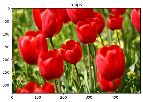
データセットから画像を取得し、それを使用してデータ増強を実演してみましょう。

get_label_name = metadata.features['label'].int2str

image, label = next(iter(train_ds))
_ = plt.imshow(image)
_ = plt.title(get_label_name(label))

2024-01-11 22:20:26.776495: W tensorflow/core/kernels/data/cache_dataset_ops.cc:858] The calling iterator did not fully read the dataset being cached. In order to avoid unexpected truncation of the dataset, the partially cached contents of the dataset  will be discarded. This can happen if you have an input pipeline similar to `dataset.cache().take(k).repeat()`. You should use `dataset.take(k).cache().repeat()` instead.

png

Keras 前処理レイヤーを使用する

リサイズとリスケール

Keras 前処理レイヤーを使用して、画像を一定の形状にサイズ変更し（tf.keras.layers.Resizing）、ピクセル値を再スケールする（tf.keras.layers.Rescaling）ことができます。

IMG_SIZE = 180

resize_and_rescale = tf.keras.Sequential([
  layers.Resizing(IMG_SIZE, IMG_SIZE),
  layers.Rescaling(1./255)
])

注意: 上記のリスケーリングレイヤーは、ピクセル値を [0,1] の範囲に標準化します。代わりに [-1,1] を用いる場合には、tf.keras.layers.Rescaling(1./127.5, offset=-1) と記述します。

次のようにして、これらのレイヤーを画像に適用した結果を可視化します。

result = resize_and_rescale(image)
_ = plt.imshow(result)

png

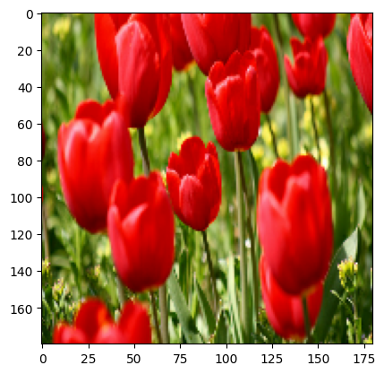
ピクセルが [0, 1] の範囲にあることを確認します。

print("Min and max pixel values:", result.numpy().min(), result.numpy().max())

Min and max pixel values: 0.0 1.0

データ増強

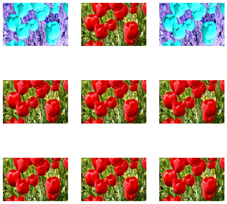
tf.keras.layers.RandomFlip や tf.keras.layers.RandomRotation などの Keras 前処理レイヤーをデータ拡張に使用することができます。

前処理レイヤーをいくつか作成し、同じ画像に繰り返して適用してみましょう。

data_augmentation = tf.keras.Sequential([
  layers.RandomFlip("horizontal_and_vertical"),
  layers.RandomRotation(0.2),
])

# Add the image to a batch.
image = tf.cast(tf.expand_dims(image, 0), tf.float32)

plt.figure(figsize=(10, 10))
for i in range(9):
  augmented_image = data_augmentation(image)
  ax = plt.subplot(3, 3, i + 1)
  plt.imshow(augmented_image[0])
  plt.axis("off")

WARNING:matplotlib.image:Clipping input data to the valid range for imshow with RGB data ([0..1] for floats or [0..255] for integers).
WARNING:matplotlib.image:Clipping input data to the valid range for imshow with RGB data ([0..1] for floats or [0..255] for integers).
WARNING:matplotlib.image:Clipping input data to the valid range for imshow with RGB data ([0..1] for floats or [0..255] for integers).
WARNING:matplotlib.image:Clipping input data to the valid range for imshow with RGB data ([0..1] for floats or [0..255] for integers).
WARNING:matplotlib.image:Clipping input data to the valid range for imshow with RGB data ([0..1] for floats or [0..255] for integers).
WARNING:matplotlib.image:Clipping input data to the valid range for imshow with RGB data ([0..1] for floats or [0..255] for integers).
WARNING:matplotlib.image:Clipping input data to the valid range for imshow with RGB data ([0..1] for floats or [0..255] for integers).
WARNING:matplotlib.image:Clipping input data to the valid range for imshow with RGB data ([0..1] for floats or [0..255] for integers).
WARNING:matplotlib.image:Clipping input data to the valid range for imshow with RGB data ([0..1] for floats or [0..255] for integers).

png

データ拡張には、tf.keras.layers.RandomContrast、tf.keras.layers.RandomCrop、tf.keras.layers.RandomZoom など、様々な前処理レイヤーを使用できます。

Keras 前処理レイヤーを使用するための 2 つのオプション

これらの前処理レイヤーを使用できる方法には 2 つありませうが、これらには重要なトレードオフが伴います。

オプション 1: 前処理レイヤーをモデルの一部にする

model = tf.keras.Sequential([
  # Add the preprocessing layers you created earlier.
  resize_and_rescale,
  data_augmentation,
  layers.Conv2D(16, 3, padding='same', activation='relu'),
  layers.MaxPooling2D(),
  # Rest of your model.
])

この場合、2 つの重要なポイントがあります。

データ増強はデバイス上で他のレイヤーと同期して実行されるため、GPU アクセラレーションの恩恵を受けることができます。
model.saveを使用してモデルをエクスポートすると、前処理レイヤーはモデルの残りの部分と一緒に保存されます。後でこのモデルをデプロイする場合、画像は自動的に（レイヤーの設定に従い）標準化されます。これにより、サーバーサイドでロジックを再実装する手間が省けます。

注意: データ拡張はテスト時には非アクティブなので、(Model.evaluate や Model.predict ではなく) Model.fit への呼び出し時にのみ、入力画像を拡張します。

オプション 2: 前処理レイヤーをデータセットに適用する

aug_ds = train_ds.map(
  lambda x, y: (resize_and_rescale(x, training=True), y))

このアプローチでは、Dataset.map を使用して、拡張画像のバッチを生成するデータセットを作成します。この場合は、

データ拡張は CPU 上で非同期に行われ、ノンブロッキングです。以下に示すように、Dataset.prefetch を使用して GPU 上でのモデルのトレーニングをデータの前処理にオーバーラップさせることができます。
この場合、Model.save を呼び出しても、前処理レイヤーはモデルと一緒にエクスポートされません。保存前にモデルに前処理レイヤーをアタッチするか、サーバー側で前処理レイヤーを再実装する必要があります。トレーニングの後、エクスポートする前に前処理レイヤーをアタッチすることができます。

1 番目のオプションの例については、画像分類チュートリアルをご覧ください。次に、2 番目のオプションを見てみましょう。

前処理レイヤーをデータセットに適用する

前に作成した前処理レイヤーを使用して、トレーニング、検証、テスト用のデータセットを構成します。また、パフォーマンス向上のために、並列読み取りとバッファ付きプリフェッチを使用してデータセットを構成し、I/O がブロックされることなくディスクからバッチを生成できるようにします。（データセットのパフォーマンスに関する詳細は、tf.data API によるパフォーマンス向上ガイドをご覧ください。）

注意: データ拡張はトレーニングセットのみに適用されます。

batch_size = 32
AUTOTUNE = tf.data.AUTOTUNE

def prepare(ds, shuffle=False, augment=False):
  # Resize and rescale all datasets.
  ds = ds.map(lambda x, y: (resize_and_rescale(x), y), 
              num_parallel_calls=AUTOTUNE)

  if shuffle:
    ds = ds.shuffle(1000)

  # Batch all datasets.
  ds = ds.batch(batch_size)

  # Use data augmentation only on the training set.
  if augment:
    ds = ds.map(lambda x, y: (data_augmentation(x, training=True), y), 
                num_parallel_calls=AUTOTUNE)

  # Use buffered prefetching on all datasets.
  return ds.prefetch(buffer_size=AUTOTUNE)

train_ds = prepare(train_ds, shuffle=True, augment=True)
val_ds = prepare(val_ds)
test_ds = prepare(test_ds)

モデルをトレーニングする

完全を期すために、準備したデータセットを使用してモデルをトレーニングします。

Sequential モデルは、それぞれに最大プールレイヤー（tf.keras.layers.MaxPooling2D）を持つ3つの畳み込みブロック（tf.keras.layers.Conv2D）で構成されます。ReLU 活性化関数（'relu'）により活性化されたユニットが 128 個ある完全に接続されたレイヤー（tf.keras.layers.Dense）があります。このモデルの精度は調整されていません（このチュートリアルの目的は、標準的なアプローチを示すことであるため）。

model = tf.keras.Sequential([
  layers.Conv2D(16, 3, padding='same', activation='relu'),
  layers.MaxPooling2D(),
  layers.Conv2D(32, 3, padding='same', activation='relu'),
  layers.MaxPooling2D(),
  layers.Conv2D(64, 3, padding='same', activation='relu'),
  layers.MaxPooling2D(),
  layers.Flatten(),
  layers.Dense(128, activation='relu'),
  layers.Dense(num_classes)
])

tf.keras.optimizers.Adam オプティマイザとtf.keras.losses.SparseCategoricalCrossentropy 損失関数を選択します。各トレーニングエポックのトレーニングと検証の精度を表示するには、Model.compile に metrics 引数を渡します。

model.compile(optimizer='adam',
              loss=tf.keras.losses.SparseCategoricalCrossentropy(from_logits=True),
              metrics=['accuracy'])

数エポック、トレーニングします。

epochs=5
history = model.fit(
  train_ds,
  validation_data=val_ds,
  epochs=epochs
)

Epoch 1/5
WARNING: All log messages before absl::InitializeLog() is called are written to STDERR
I0000 00:00:1705011632.174898 1015219 device_compiler.h:186] Compiled cluster using XLA!  This line is logged at most once for the lifetime of the process.
92/92 [==============================] - 9s 46ms/step - loss: 1.3657 - accuracy: 0.4067 - val_loss: 1.1159 - val_accuracy: 0.5531
Epoch 2/5
92/92 [==============================] - 2s 21ms/step - loss: 1.0734 - accuracy: 0.5654 - val_loss: 0.9760 - val_accuracy: 0.6567
Epoch 3/5
92/92 [==============================] - 2s 21ms/step - loss: 0.9780 - accuracy: 0.6097 - val_loss: 1.0353 - val_accuracy: 0.5749
Epoch 4/5
92/92 [==============================] - 2s 21ms/step - loss: 0.9035 - accuracy: 0.6339 - val_loss: 0.9541 - val_accuracy: 0.6349
Epoch 5/5
92/92 [==============================] - 2s 21ms/step - loss: 0.8713 - accuracy: 0.6540 - val_loss: 0.9970 - val_accuracy: 0.6349

loss, acc = model.evaluate(test_ds)
print("Accuracy", acc)

12/12 [==============================] - 1s 7ms/step - loss: 0.9701 - accuracy: 0.6158
Accuracy 0.6158038377761841

カスタムデータ増強

また、カスタムデータ拡張レイヤーを作成することもできます。

このセクションでは、これを行うための 2 つの方法を説明します。

まず、tf.keras.layers.Lambda レイヤーを作成します。簡潔なコードを書くには良い方法です。
次に、subclassing を介して新しいレイヤーを記述します。こうすることで、さらに制御できるようになります。

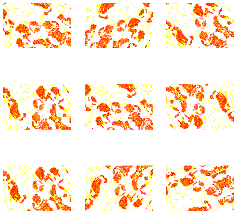
どちらのレイヤーも、確率に従って、画像の色をランダムに反転します。

def random_invert_img(x, p=0.5):
  if  tf.random.uniform([]) < p:
    x = (255-x)
  else:
    x
  return x

def random_invert(factor=0.5):
  return layers.Lambda(lambda x: random_invert_img(x, factor))

random_invert = random_invert()

plt.figure(figsize=(10, 10))
for i in range(9):
  augmented_image = random_invert(image)
  ax = plt.subplot(3, 3, i + 1)
  plt.imshow(augmented_image[0].numpy().astype("uint8"))
  plt.axis("off")

png

次に、サブクラス化してカスタムレイヤーを実装します。

class RandomInvert(layers.Layer):
  def __init__(self, factor=0.5, **kwargs):
    super().__init__(**kwargs)
    self.factor = factor

  def call(self, x):
    return random_invert_img(x)

_ = plt.imshow(RandomInvert()(image)[0])

WARNING:matplotlib.image:Clipping input data to the valid range for imshow with RGB data ([0..1] for floats or [0..255] for integers).

png

どちらのレイヤーも、上記 1 と 2 のオプションで説明した使用が可能です。

tf.image を使用する

上記の Keras 前処理ユーティリティは便利ではありますが、より細かい制御には、tf.data や tf.image を使用して独自のデータ拡張パイプラインやレイヤーを書くことができます。（また、TensorFlow Addons 画像: 演算および TensorFlow I/O: 色空間の変換もご覧ください。）

花のデータセットは、前にデータ拡張で構成したので、再インポートして最初からやり直しましょう。

(train_ds, val_ds, test_ds), metadata = tfds.load(
    'tf_flowers',
    split=['train[:80%]', 'train[80%:90%]', 'train[90%:]'],
    with_info=True,
    as_supervised=True,
)

作業に必要な画像を取得します。

image, label = next(iter(train_ds))
_ = plt.imshow(image)
_ = plt.title(get_label_name(label))

2024-01-11 22:20:51.328796: W tensorflow/core/kernels/data/cache_dataset_ops.cc:858] The calling iterator did not fully read the dataset being cached. In order to avoid unexpected truncation of the dataset, the partially cached contents of the dataset  will be discarded. This can happen if you have an input pipeline similar to `dataset.cache().take(k).repeat()`. You should use `dataset.take(k).cache().repeat()` instead.

png

以下の関数を使用して元の画像と拡張画像を並べて視覚化し、比較してみましょう。

def visualize(original, augmented):
  fig = plt.figure()
  plt.subplot(1,2,1)
  plt.title('Original image')
  plt.imshow(original)

  plt.subplot(1,2,2)
  plt.title('Augmented image')
  plt.imshow(augmented)

データ増強

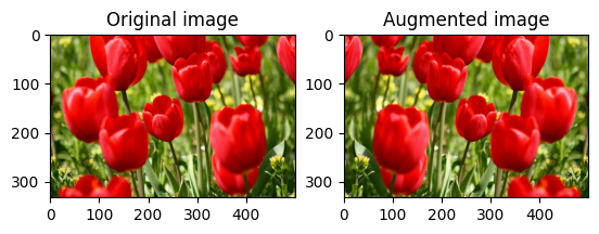
画像をフリップする

tf.image.flip_left_right を使って、画像を縦方向または横方向に反転します。

flipped = tf.image.flip_left_right(image)
visualize(image, flipped)

png

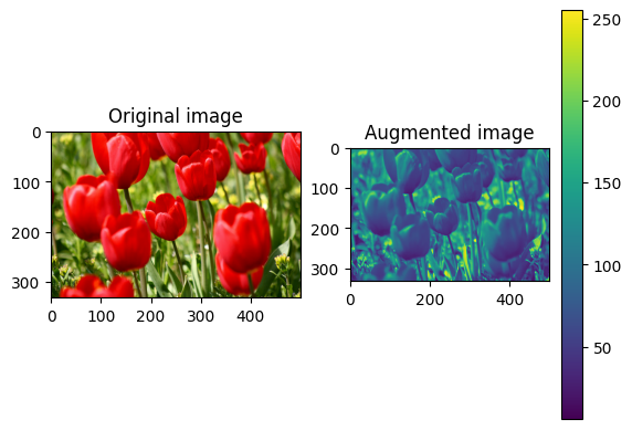
画像をグレースケールにする

tf.image.rgb_to_grayscale を使って、画像をグレースケールにできます。

grayscaled = tf.image.rgb_to_grayscale(image)
visualize(image, tf.squeeze(grayscaled))
_ = plt.colorbar()

png

画像の彩度を処理する

tf.image.adjust_saturation を使用し、彩度係数を指定して画像の彩度を操作します。

saturated = tf.image.adjust_saturation(image, 3)
visualize(image, saturated)

png

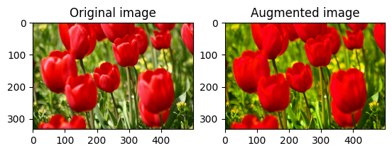
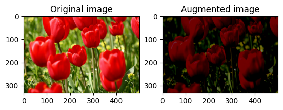
画像の明るさを変更する

tf.image.adjust_brightness を使用し、明度係数を指定して画像の明度を変更します。

bright = tf.image.adjust_brightness(image, 0.4)
visualize(image, bright)

png

画像を中央でトリミングする

tf.image.central_crop を使用して、画像の中央から希望する部分までをトリミングします。

cropped = tf.image.central_crop(image, central_fraction=0.5)
visualize(image, cropped)

png

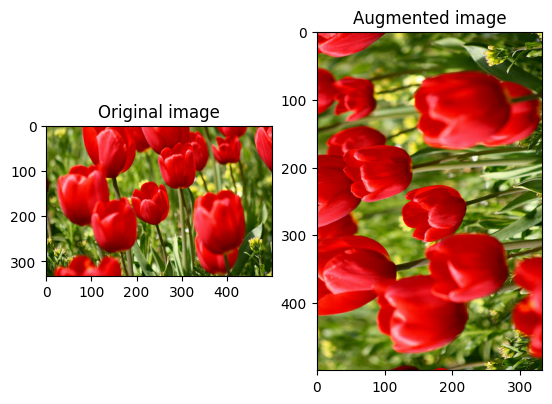
画像を回転させる

tf.image.rot90 を使用して、画像を 90 度回転させます。

rotated = tf.image.rot90(image)
visualize(image, rotated)

png

ランダム変換

警告: ランダム画像演算には tf.image.random* および tf.image.stateless_random* の 2 つのセットがあります。tf.image.random* 演算は、TF 1.x の古い RNG を使用するため、使用することは強くお勧めしません。代わりに、このチュートリアルで紹介したランダム画像演算を使用してください。詳細については、乱数の生成を参照してください。

画像にランダムな変換を適用すると、データセットの一般化と拡張にさらに役立ちます。現在の tf.image は、次の 8 つのランダム画像演算 (ops) を提供します。

これらのランダム画像演算は機能的であり、出力は入力にのみ依存します。これにより、高性能で決定論的な入力パイプラインで簡単に使用できるようになります。各ステップで seed 値を入力する必要があります。同じ seedを指定すると、呼び出された回数に関係なく、同じ結果が返されます。

注意: seed は、形状が (2,) の Tensor で、値は任意の整数です。

以降のセクションでは、次のことを行います。

ランダム画像演算を使用して画像を変換する例を見る。
ランダム変換をトレーニングデータセットに適用する方法を示す。

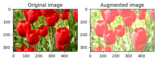
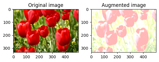
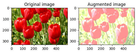
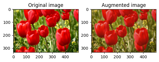
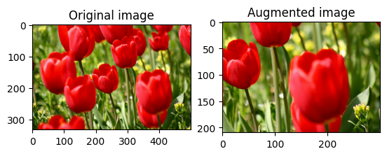
画像の明るさをランダムに変更する

tf.image.stateless_random_brightness を使用し、明度係数と seed を指定して、image の明度をランダムに変更します。明度係数は、[-max_delta, max_delta) の範囲でランダムに選択され、指定された seed に関連付けられます。

for i in range(3):
  seed = (i, 0)  # tuple of size (2,)
  stateless_random_brightness = tf.image.stateless_random_brightness(
      image, max_delta=0.95, seed=seed)
  visualize(image, stateless_random_brightness)

png

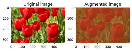
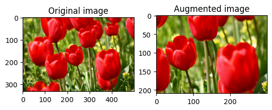
画像のコントラストをランダムに変更する

tf.image.stateless_random_contrast を使用し、コントラスト範囲と seed を指定して、image のコントラストをランダムに変更します。コントラスト範囲は、[lower, upper] の間隔でランダムに選択され、指定された seed に関連付けられます。

for i in range(3):
  seed = (i, 0)  # tuple of size (2,)
  stateless_random_contrast = tf.image.stateless_random_contrast(
      image, lower=0.1, upper=0.9, seed=seed)
  visualize(image, stateless_random_contrast)

png

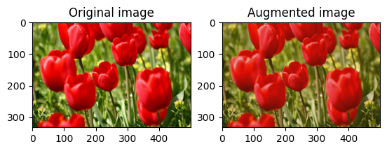
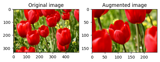
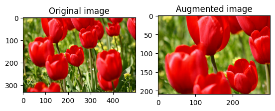
ランダムに画像をトリミングする

tf.image.stateless_random_crop を使用し、ターゲットの size と seed を指定して image をランダムにトリミングします。image から切り取られる部分は、ランダムに選択されたオフセットにあり、指定された seed に関連付けられています。

for i in range(3):
  seed = (i, 0)  # tuple of size (2,)
  stateless_random_crop = tf.image.stateless_random_crop(
      image, size=[210, 300, 3], seed=seed)
  visualize(image, stateless_random_crop)

png

データ増強をデータセットに適用する

前に説明したように、Dataset.map を使用してデータセットにデータ拡張を適用します。

(train_datasets, val_ds, test_ds), metadata = tfds.load(
    'tf_flowers',
    split=['train[:80%]', 'train[80%:90%]', 'train[90%:]'],
    with_info=True,
    as_supervised=True,
)

次に、画像のサイズ変更と再スケーリングのためのユーティリティ関数を定義します。この関数は、データセット内の画像のサイズとスケールを統一するために使用されます。

def resize_and_rescale(image, label):
  image = tf.cast(image, tf.float32)
  image = tf.image.resize(image, [IMG_SIZE, IMG_SIZE])
  image = (image / 255.0)
  return image, label

また、画像にランダム変換を適用できる augment 関数も定義します。この関数は、次のステップのデータセットで使用されます。

def augment(image_label, seed):
  image, label = image_label
  image, label = resize_and_rescale(image, label)
  image = tf.image.resize_with_crop_or_pad(image, IMG_SIZE + 6, IMG_SIZE + 6)
  # Make a new seed.
  new_seed = tf.random.split(seed, num=1)[0, :]
  # Random crop back to the original size.
  image = tf.image.stateless_random_crop(
      image, size=[IMG_SIZE, IMG_SIZE, 3], seed=seed)
  # Random brightness.
  image = tf.image.stateless_random_brightness(
      image, max_delta=0.5, seed=new_seed)
  image = tf.clip_by_value(image, 0, 1)
  return image, label

オプション 1: tf.data.experimental.Counte を使用する

tf.data.experimental.Counter オブジェクト (counter と呼ぶ) を作成し、(counter, counter) を含むデータセットを zip します。これにより、データセット内の各画像が、counter に基づいて（一意の値形状 (2,)）に関連付けられるようになります。これは後で、ランダム変換の seed 値として augment 関数に渡されます。

# Create a `Counter` object and `Dataset.zip` it together with the training set.
counter = tf.data.experimental.Counter()
train_ds = tf.data.Dataset.zip((train_datasets, (counter, counter)))

WARNING:tensorflow:From /tmpfs/tmp/ipykernel_1015044/587852618.py:2: CounterV2 (from tensorflow.python.data.experimental.ops.counter) is deprecated and will be removed in a future version.
Instructions for updating:
Use `tf.data.Dataset.counter(...)` instead.
WARNING:tensorflow:From /tmpfs/tmp/ipykernel_1015044/587852618.py:2: CounterV2 (from tensorflow.python.data.experimental.ops.counter) is deprecated and will be removed in a future version.
Instructions for updating:
Use `tf.data.Dataset.counter(...)` instead.

augment 関数をトレーニングデータセットにマッピングします。

train_ds = (
    train_ds
    .shuffle(1000)
    .map(augment, num_parallel_calls=AUTOTUNE)
    .batch(batch_size)
    .prefetch(AUTOTUNE)
)

val_ds = (
    val_ds
    .map(resize_and_rescale, num_parallel_calls=AUTOTUNE)
    .batch(batch_size)
    .prefetch(AUTOTUNE)
)

test_ds = (
    test_ds
    .map(resize_and_rescale, num_parallel_calls=AUTOTUNE)
    .batch(batch_size)
    .prefetch(AUTOTUNE)
)

オプション 2: `tf.random.Generator` を使用する

seed の初期値で tf.random.Generator オブジェクトを作成します。同じジェネレータオブジェクトに make_seeds 関数を呼び出すと、必ず新しい一意の seed 値が返されます。
ラッパー関数を 1) make_seeds 関数を呼び出し、2) 新たに生成された seed 値を augment 関数に渡してランダム変換を行うように定義します。

注意: tf.random.Generator オブジェクトは RNG 状態を tf.Variable に格納するため、checkpoint または SavedModel として保存できます。詳細につきましては、乱数の生成を参照してください。

# Create a generator.
rng = tf.random.Generator.from_seed(123, alg='philox')

# Create a wrapper function for updating seeds.
def f(x, y):
  seed = rng.make_seeds(2)[0]
  image, label = augment((x, y), seed)
  return image, label

ラッパー関数 f をトレーニングデータセットにマッピングし、resize_and_rescale 関数を検証セットとテストセットにマッピングします。

train_ds = (
    train_datasets
    .shuffle(1000)
    .map(f, num_parallel_calls=AUTOTUNE)
    .batch(batch_size)
    .prefetch(AUTOTUNE)
)

val_ds = (
    val_ds
    .map(resize_and_rescale, num_parallel_calls=AUTOTUNE)
    .batch(batch_size)
    .prefetch(AUTOTUNE)
)

test_ds = (
    test_ds
    .map(resize_and_rescale, num_parallel_calls=AUTOTUNE)
    .batch(batch_size)
    .prefetch(AUTOTUNE)
)

前に示したように、これらのデータセットはモデルのトレーニングに使用が可能です。

次のステップ

このチュートリアルでは、Keras 前処理レイヤーと tf.image を使用したデータ拡張を説明しました。

モデル内に前処理レイヤーを含める方法については、画像の分類チュートリアルをご覧ください。
前処理レイヤーでテキストを分類する方法にも関心がある場合は、基本的なテキスト分類チュートリアルをご覧ください。
tf.data については、こちらのガイドでもさらに詳しく学習できます。パフォーマンスを向上させる入力パイプラインの構成方法については、こちらをご覧ください。

データ増強

概要

セットアップ

データセットをダウンロードする

Keras 前処理レイヤーを使用する

リサイズとリスケール

データ増強

Keras 前処理レイヤーを使用するための 2 つのオプション

オプション 1: 前処理レイヤーをモデルの一部にする

オプション 2: 前処理レイヤーをデータセットに適用する

前処理レイヤーをデータセットに適用する

モデルをトレーニングする

カスタムデータ増強

tf.image を使用する

データ増強

画像をフリップする

画像をグレースケールにする

画像の彩度を処理する

画像の明るさを変更する

画像を中央でトリミングする

画像を回転させる

ランダム変換

画像の明るさをランダムに変更する

画像のコントラストをランダムに変更する

ランダムに画像をトリミングする

データ増強をデータセットに適用する

オプション 1: tf.data.experimental.Counte を使用する

オプション 2: tf.random.Generator を使用する

次のステップ

オプション 2: `tf.random.Generator` を使用する