
 在 GitHub 中查看源代码 在 GitHub 中查看源代码 |
TensorFlow Hub 是预训练的 TensorFlow 模型的仓库。
此教程演示了如何执行以下操作:
- 将来自 TensorFlow Hub 的模型与
tf.keras结合使用 - 使用来自 TensorFlow Hub 的图像分类模型
- 进行简单的迁移学习,针对您自己的图像类微调模型
设置
import numpy as np
import time

import PIL.Image as Image
import matplotlib.pylab as plt

import tensorflow as tf
import tensorflow_hub as hub

import datetime

%load_ext tensorboard
2023-11-07 23:03:51.866811: E external/local_xla/xla/stream_executor/cuda/cuda_dnn.cc:9261] Unable to register cuDNN factory: Attempting to register factory for plugin cuDNN when one has already been registered
2023-11-07 23:03:51.866865: E external/local_xla/xla/stream_executor/cuda/cuda_fft.cc:607] Unable to register cuFFT factory: Attempting to register factory for plugin cuFFT when one has already been registered
2023-11-07 23:03:51.868626: E external/local_xla/xla/stream_executor/cuda/cuda_blas.cc:1515] Unable to register cuBLAS factory: Attempting to register factory for plugin cuBLAS when one has already been registered
ImageNet 分类器
您将首先使用预训练的分类器模型获取图像并预测它是什么图像 - 无需训练!
下载分类器
从 TensorFlow Hub 中选择一个 MobileNetV2 预训练模型,并将其封装为带有 hub.KerasLayer 的 hub.KerasLayer 层。可以在这里使用任何来自 TensorFlow Hub 的兼容的图像分类器模型,包括下面下拉列表中提供的示例。
mobilenet_v2 ="https://tfhub.dev/google/tf2-preview/mobilenet_v2/classification/4"
inception_v3 = "https://tfhub.dev/google/imagenet/inception_v3/classification/5"

classifier_model = mobilenet_v2
IMAGE_SHAPE = (224, 224)

classifier = tf.keras.Sequential([
    hub.KerasLayer(classifier_model, input_shape=IMAGE_SHAPE+(3,))
])
对单个图像运行分类器
下载要在模型上尝试的单个图像。
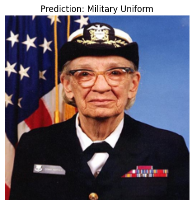
grace_hopper = tf.keras.utils.get_file('image.jpg','https://storage.googleapis.com/download.tensorflow.org/example_images/grace_hopper.jpg')
grace_hopper = Image.open(grace_hopper).resize(IMAGE_SHAPE)
grace_hopper
Downloading data from https://storage.googleapis.com/download.tensorflow.org/example_images/grace_hopper.jpg
61306/61306 [==============================] - 0s 0us/step

grace_hopper = np.array(grace_hopper)/255.0
grace_hopper.shape
(224, 224, 3)
添加批量维度(使用 np.newaxis)并将图像传递给模型:
result = classifier.predict(grace_hopper[np.newaxis, ...])
result.shape
1/1 [==============================] - 2s 2s/step
(1, 1001)
结果是一个 1001 元素的 logits 向量,同时对图像属于每个类别的概率进行评分。
顶部类 ID 可以通过 tf.math.argmax 找到:
predicted_class = tf.math.argmax(result[0], axis=-1)
predicted_class
<tf.Tensor: shape=(), dtype=int64, numpy=653>
解码预测
获取 predicted_class ID(例如 653)并获取 ImageNet 数据集标签以解码预测:
labels_path = tf.keras.utils.get_file('ImageNetLabels.txt','https://storage.googleapis.com/download.tensorflow.org/data/ImageNetLabels.txt')
imagenet_labels = np.array(open(labels_path).read().splitlines())
Downloading data from https://storage.googleapis.com/download.tensorflow.org/data/ImageNetLabels.txt
10484/10484 [==============================] - 0s 0us/step
plt.imshow(grace_hopper)
plt.axis('off')
predicted_class_name = imagenet_labels[predicted_class]
_ = plt.title("Prediction: " + predicted_class_name.title())
简单的迁移学习
但是,如果您想使用自己的数据集创建一个自定义分类器,但该数据集的类未包含在原始 ImageNet 数据集中(预训练模型已基于该数据集进行训练),此时该如何处理?
为此,您可以:
- 从 TensorFlow Hub 中选择一个预训练模型;
- 重新训练顶部(最后一个)层以识别自定义数据集中的类。
数据集
在本例中,您将使用 TensorFlow 花卉数据集:
import pathlib

data_file = tf.keras.utils.get_file(
  'flower_photos.tgz',
  'https://storage.googleapis.com/download.tensorflow.org/example_images/flower_photos.tgz',
  cache_dir='.',
   extract=True)

data_root = pathlib.Path(data_file).with_suffix('')
Downloading data from https://storage.googleapis.com/download.tensorflow.org/example_images/flower_photos.tgz
228813984/228813984 [==============================] - 1s 0us/step
首先,使用 tf.keras.utils.image_dataset_from_directory 将磁盘上的图像数据加载到模型中,这将生成一个 tf.data.Dataset:
batch_size = 32
img_height = 224
img_width = 224

train_ds = tf.keras.utils.image_dataset_from_directory(
  str(data_root),
  validation_split=0.2,
  subset="training",
  seed=123,
  image_size=(img_height, img_width),
  batch_size=batch_size
)

val_ds = tf.keras.utils.image_dataset_from_directory(
  str(data_root),
  validation_split=0.2,
  subset="validation",
  seed=123,
  image_size=(img_height, img_width),
  batch_size=batch_size
)
Found 3670 files belonging to 5 classes.
Using 2936 files for training.
Found 3670 files belonging to 5 classes.
Using 734 files for validation.
花卉数据集有五个类。
class_names = np.array(train_ds.class_names)
print(class_names)
['daisy' 'dandelion' 'roses' 'sunflowers' 'tulips']
其次,由于 TensorFlow Hub 对图像模型的约定是期望浮点输入在 [0, 1] 范围内,因此使用 tf.keras.layers.Rescaling 预处理层来实现这一点。
注:您还可以在模型中包含 tf.keras.layers.Rescaling 层。有关权衡的讨论,请参阅使用预处理层指南。
normalization_layer = tf.keras.layers.Rescaling(1./255)
train_ds = train_ds.map(lambda x, y: (normalization_layer(x), y)) # Where x—images, y—labels.
val_ds = val_ds.map(lambda x, y: (normalization_layer(x), y)) # Where x—images, y—labels.
第三,通过使用 Dataset.prefetch 的缓冲预提取来完成输入流水线,这样您就可以从磁盘产生数据而不会出现 I/O 阻塞问题。
这些是加载数据时应该使用的一些最重要的 tf.data 方法。感兴趣的读者可以在使用 tf.data API 获得更高性能指南中了解有关它们的更多信息,以及如何将数据缓存到磁盘和其他技术。
AUTOTUNE = tf.data.AUTOTUNE
train_ds = train_ds.cache().prefetch(buffer_size=AUTOTUNE)
val_ds = val_ds.cache().prefetch(buffer_size=AUTOTUNE)
for image_batch, labels_batch in train_ds:
  print(image_batch.shape)
  print(labels_batch.shape)
  break
(32, 224, 224, 3)
(32,)
2023-11-07 23:04:06.599504: W tensorflow/core/kernels/data/cache_dataset_ops.cc:858] The calling iterator did not fully read the dataset being cached. In order to avoid unexpected truncation of the dataset, the partially cached contents of the dataset  will be discarded. This can happen if you have an input pipeline similar to `dataset.cache().take(k).repeat()`. You should use `dataset.take(k).cache().repeat()` instead.
对一批图像运行分类器
接下来,对图像批次运行分类器。
result_batch = classifier.predict(train_ds)
92/92 [==============================] - 6s 41ms/step
predicted_class_names = imagenet_labels[tf.math.argmax(result_batch, axis=-1)]
predicted_class_names
array(['daisy', 'coral fungus', 'rapeseed', ..., 'daisy', 'daisy',
       'birdhouse'], dtype='<U30')
检查这些预测值与图像的对应关系:
plt.figure(figsize=(10,9))
plt.subplots_adjust(hspace=0.5)
for n in range(30):
  plt.subplot(6,5,n+1)
  plt.imshow(image_batch[n])
  plt.title(predicted_class_names[n])
  plt.axis('off')
_ = plt.suptitle("ImageNet predictions")
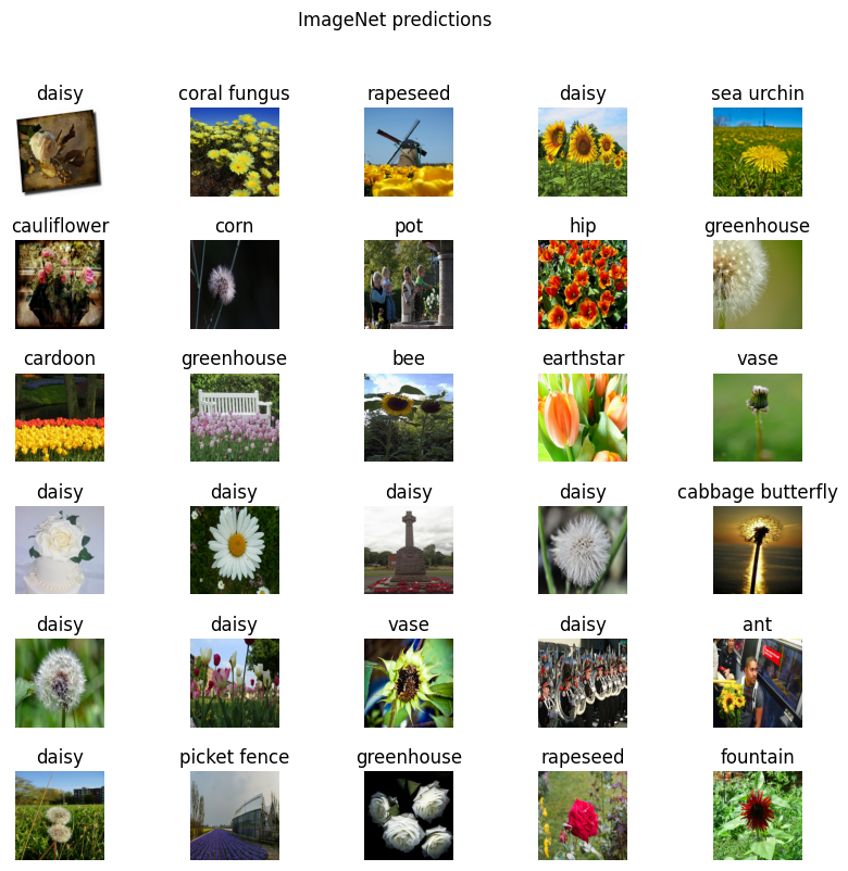
注:所有图像均获得 CC-BY 许可,创作者列于 LICENSE.txt 文件中。
结果远远不够完美,但考虑到这些类并不是训练模型时所用的类(“雏菊”除外),结果也算合理。
下载无头模型
TensorFlow Hub 还可以分发没有顶部分类层的模型。这些模型可用于轻松执行迁移学习。
从 TensorFlow Hub 中选择一个 MobileNetV2 预训练模型。可以在这里使用任何来自 TensorFlow Hub 的兼容的图像特征向量模型,包括下拉菜单中的示例。
mobilenet_v2 = "https://tfhub.dev/google/tf2-preview/mobilenet_v2/feature_vector/4"
inception_v3 = "https://tfhub.dev/google/tf2-preview/inception_v3/feature_vector/4"

feature_extractor_model = mobilenet_v2
通过将预训练模型包装为带有 hub.KerasLayer 的 Keras 层来创建特征提取器。使用 trainable=False 参数冻结变量,以便训练只修改新的分类器层:
feature_extractor_layer = hub.KerasLayer(
    feature_extractor_model,
    input_shape=(224, 224, 3),
    trainable=False)
特征提取器会为每个图像返回一个长度为 1280 的向量(在此示例中,图像批量大小保持为 32):
feature_batch = feature_extractor_layer(image_batch)
print(feature_batch.shape)
(32, 1280)
附加分类头
为了完成模型,将特征提取器层包装在一个 tf.keras.Sequential 模型中,并添加一个全连接层进行分类:
num_classes = len(class_names)

model = tf.keras.Sequential([
  feature_extractor_layer,
  tf.keras.layers.Dense(num_classes)
])

model.summary()
Model: "sequential_1"
_________________________________________________________________
 Layer (type)                Output Shape              Param #
=================================================================
 keras_layer_1 (KerasLayer)  (None, 1280)              2257984

 dense (Dense)               (None, 5)                 6405

=================================================================
Total params: 2264389 (8.64 MB)
Trainable params: 6405 (25.02 KB)
Non-trainable params: 2257984 (8.61 MB)
_________________________________________________________________
predictions = model(image_batch)
predictions.shape
TensorShape([32, 5])
训练模型
使用 Model.compile 配置训练过程并添加 tf.keras.callbacks.TensorBoard 回调来创建和存储日志:
model.compile(
  optimizer=tf.keras.optimizers.Adam(),
  loss=tf.keras.losses.SparseCategoricalCrossentropy(from_logits=True),
  metrics=['acc'])

log_dir = "logs/fit/" + datetime.datetime.now().strftime("%Y%m%d-%H%M%S")
tensorboard_callback = tf.keras.callbacks.TensorBoard(
    log_dir=log_dir,
    histogram_freq=1) # Enable histogram computation for every epoch.
现在使用 Model.fit 方法来训练模型。
为了缩短本示例,您将只训练 10 个周期。为了稍后在 TensorBoard 中呈现训练进度,为日志创建并存储一个 TensorBoard 回调。
NUM_EPOCHS = 10

history = model.fit(train_ds,
                    validation_data=val_ds,
                    epochs=NUM_EPOCHS,
                    callbacks=tensorboard_callback)
Epoch 1/10
WARNING: All log messages before absl::InitializeLog() is called are written to STDERR
I0000 00:00:1699398259.942138  504335 device_compiler.h:186] Compiled cluster using XLA!  This line is logged at most once for the lifetime of the process.
92/92 [==============================] - 12s 88ms/step - loss: 0.7662 - acc: 0.7180 - val_loss: 0.4414 - val_acc: 0.8597
Epoch 2/10
92/92 [==============================] - 6s 67ms/step - loss: 0.3665 - acc: 0.8770 - val_loss: 0.3553 - val_acc: 0.8801
Epoch 3/10
92/92 [==============================] - 6s 67ms/step - loss: 0.2873 - acc: 0.9087 - val_loss: 0.3214 - val_acc: 0.8937
Epoch 4/10
92/92 [==============================] - 6s 67ms/step - loss: 0.2397 - acc: 0.9288 - val_loss: 0.3042 - val_acc: 0.8992
Epoch 5/10
92/92 [==============================] - 6s 66ms/step - loss: 0.2058 - acc: 0.9401 - val_loss: 0.2946 - val_acc: 0.9019
Epoch 6/10
92/92 [==============================] - 6s 67ms/step - loss: 0.1797 - acc: 0.9503 - val_loss: 0.2888 - val_acc: 0.9046
Epoch 7/10
92/92 [==============================] - 6s 67ms/step - loss: 0.1587 - acc: 0.9612 - val_loss: 0.2851 - val_acc: 0.9074
Epoch 8/10
92/92 [==============================] - 6s 66ms/step - loss: 0.1414 - acc: 0.9670 - val_loss: 0.2827 - val_acc: 0.9114
Epoch 9/10
92/92 [==============================] - 6s 67ms/step - loss: 0.1268 - acc: 0.9721 - val_loss: 0.2810 - val_acc: 0.9101
Epoch 10/10
92/92 [==============================] - 6s 67ms/step - loss: 0.1143 - acc: 0.9762 - val_loss: 0.2798 - val_acc: 0.9114
启动 TensorBoard 以查看指标如何随每个周期变化并跟踪其他标量值:
%tensorboard --logdir logs/fit
![]()
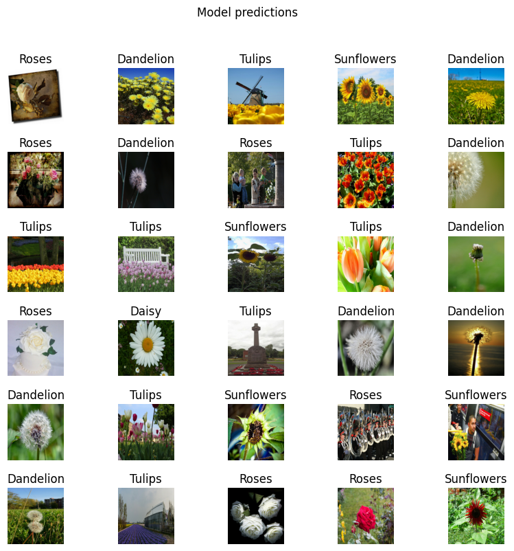
检查预测值
从模型预测中获取类名的有序列表:
predicted_batch = model.predict(image_batch)
predicted_id = tf.math.argmax(predicted_batch, axis=-1)
predicted_label_batch = class_names[predicted_id]
print(predicted_label_batch)
1/1 [==============================] - 0s 497ms/step
['roses' 'dandelion' 'tulips' 'sunflowers' 'dandelion' 'roses' 'dandelion'
 'roses' 'tulips' 'dandelion' 'tulips' 'tulips' 'sunflowers' 'tulips'
 'dandelion' 'roses' 'daisy' 'tulips' 'dandelion' 'dandelion' 'dandelion'
 'tulips' 'sunflowers' 'roses' 'sunflowers' 'dandelion' 'tulips' 'roses'
 'roses' 'sunflowers' 'tulips' 'sunflowers']
绘制模型预测:
plt.figure(figsize=(10,9))
plt.subplots_adjust(hspace=0.5)

for n in range(30):
  plt.subplot(6,5,n+1)
  plt.imshow(image_batch[n])
  plt.title(predicted_label_batch[n].title())
  plt.axis('off')
_ = plt.suptitle("Model predictions")

导出并重新加载模型
现在您已经训练了模型,将其导出为 SavedModel 以供稍后使用。
t = time.time()

export_path = "/tmp/saved_models/{}".format(int(t))
model.save(export_path)

export_path
INFO:tensorflow:Assets written to: /tmp/saved_models/1699398325/assets
INFO:tensorflow:Assets written to: /tmp/saved_models/1699398325/assets
'/tmp/saved_models/1699398325'
现在,确认我们可以重新加载该模型,并且它仍会给出相同的结果:
reloaded = tf.keras.models.load_model(export_path)
result_batch = model.predict(image_batch)
reloaded_result_batch = reloaded.predict(image_batch)
1/1 [==============================] - 0s 69ms/step
1/1 [==============================] - 1s 561ms/step
abs(reloaded_result_batch - result_batch).max()
0.0
reloaded_predicted_id = tf.math.argmax(reloaded_result_batch, axis=-1)
reloaded_predicted_label_batch = class_names[reloaded_predicted_id]
print(reloaded_predicted_label_batch)
['roses' 'dandelion' 'tulips' 'sunflowers' 'dandelion' 'roses' 'dandelion'
 'roses' 'tulips' 'dandelion' 'tulips' 'tulips' 'sunflowers' 'tulips'
 'dandelion' 'roses' 'daisy' 'tulips' 'dandelion' 'dandelion' 'dandelion'
 'tulips' 'sunflowers' 'roses' 'sunflowers' 'dandelion' 'tulips' 'roses'
 'roses' 'sunflowers' 'tulips' 'sunflowers']
plt.figure(figsize=(10,9))
plt.subplots_adjust(hspace=0.5)
for n in range(30):
  plt.subplot(6,5,n+1)
  plt.imshow(image_batch[n])
  plt.title(reloaded_predicted_label_batch[n].title())
  plt.axis('off')
_ = plt.suptitle("Model predictions")
后续步骤
您可以使用 SavedModel 加载以进行推断或将其转换为 TensorFlow Lite 模型(用于设备端机器学习)或 TensorFlow.js 模型(用于 JavaScript 中的机器学习)。
探索更多教程,了解如何在图像、文本、音频和视频任务中使用 TensorFlow Hub 中的预训练模型。