
|
|
|
 View source on GitHub View source on GitHub
|
|
このテキスト分類チュートリアルでは、感情分析のために IMDB 映画レビュー大型データセット を使って リカレントニューラルネットワーク を訓練します。
設定
!pip install tf-nightly
import tensorflow_datasets as tfds
import tensorflow as tf
2022-12-14 23:30:29.636980: E tensorflow/tsl/lib/monitoring/collection_registry.cc:81] Cannot register 2 metrics with the same name: /tensorflow/core/bfc_allocator_delay
matplotlib をインポートしグラフを描画するためのヘルパー関数を作成します。
import matplotlib.pyplot as plt

def plot_graphs(history, metric):
  plt.plot(history.history[metric])
  plt.plot(history.history['val_'+metric], '')
  plt.xlabel("Epochs")
  plt.ylabel(metric)
  plt.legend([metric, 'val_'+metric])
  plt.show()
入力パイプラインの設定
IMDB 映画レビュー大型データセットは二値分類データセットです。すべてのレビューは、好意的(positive) または 非好意的(negative) のいずれかの感情を含んでいます。
TFDS を使ってこのデータセットをダウンロードします。
dataset, info = tfds.load('imdb_reviews/subwords8k', with_info=True,
                          as_supervised=True)
train_examples, test_examples = dataset['train'], dataset['test']
WARNING:absl:TFDS datasets with text encoding are deprecated and will be removed in a future version. Instead, you should use the plain text version and tokenize the text using `tensorflow_text` (See: https://www.tensorflow.org/tutorials/tensorflow_text/intro#tfdata_example)
このデータセットの info には、エンコーダー(tfds.features.text.SubwordTextEncoder) が含まれています。
encoder = info.features['text'].encoder
print('Vocabulary size: {}'.format(encoder.vocab_size))
Vocabulary size: 8185
このテキストエンコーダーは、任意の文字列を可逆的にエンコードします。必要であればバイトエンコーディングにフォールバックします。
sample_string = 'Hello TensorFlow.'

encoded_string = encoder.encode(sample_string)
print('Encoded string is {}'.format(encoded_string))

original_string = encoder.decode(encoded_string)
print('The original string: "{}"'.format(original_string))
Encoded string is [4025, 222, 6307, 2327, 4043, 2120, 7975]
The original string: "Hello TensorFlow."
assert original_string == sample_string
for index in encoded_string:
  print('{} ----> {}'.format(index, encoder.decode([index])))
4025 ----> Hell
222 ----> o
6307 ----> Ten
2327 ----> sor
4043 ----> Fl
2120 ----> ow
7975 ----> .
訓練用データの準備
次に、これらのエンコード済み文字列をバッチ化します。padded_batch メソッドを使ってバッチ中の一番長い文字列の長さにゼロパディングを行います。
BUFFER_SIZE = 10000
BATCH_SIZE = 64
train_dataset = (train_examples
                 .shuffle(BUFFER_SIZE)
                 .padded_batch(BATCH_SIZE, padded_shapes=([None],[])))

test_dataset = (test_examples
                .padded_batch(BATCH_SIZE,  padded_shapes=([None],[])))
train_dataset = (train_examples
                 .shuffle(BUFFER_SIZE)
                 .padded_batch(BATCH_SIZE))

test_dataset = (test_examples
                .padded_batch(BATCH_SIZE))
モデルの作成
tf.keras.Sequential モデルを構築しましょう。最初に Embedding レイヤーから始めます。Embedding レイヤーは単語一つに対して一つのベクトルを収容します。呼び出しを受けると、Embedding レイヤーは単語のインデックスのシーケンスを、ベクトルのシーケンスに変換します。これらのベクトルは訓練可能です。(十分なデータで)訓練されたあとは、おなじような意味をもつ単語は、しばしばおなじようなベクトルになります。
このインデックス参照は、ワンホットベクトルを tf.keras.layers.Dense レイヤーを使って行うおなじような演算に比べてずっと効率的です。
リカレントニューラルネットワーク(RNN)は、シーケンスの入力を要素を一つずつ扱うことで処理します。RNN は、あるタイムステップでの出力を次のタイムステップの入力へと、次々に渡していきます。
RNN レイヤーとともに、tf.keras.layers.Bidirectional ラッパーを使用することができます。このラッパーは、入力を RNN 層の順方向と逆方向に伝え、その後出力を結合します。これにより、RNN は長期的な依存関係を学習できます。
model = tf.keras.Sequential([
    tf.keras.layers.Embedding(encoder.vocab_size, 64),
    tf.keras.layers.Bidirectional(tf.keras.layers.LSTM(64)),
    tf.keras.layers.Dense(64, activation='relu'),
    tf.keras.layers.Dense(1)
])
訓練プロセスを定義するため、Keras モデルをコンパイルします。
model.compile(loss=tf.keras.losses.BinaryCrossentropy(from_logits=True),
              optimizer=tf.keras.optimizers.Adam(1e-4),
              metrics=['accuracy'])
モデルの訓練
history = model.fit(train_dataset, epochs=10,
                    validation_data=test_dataset,
                    validation_steps=30)
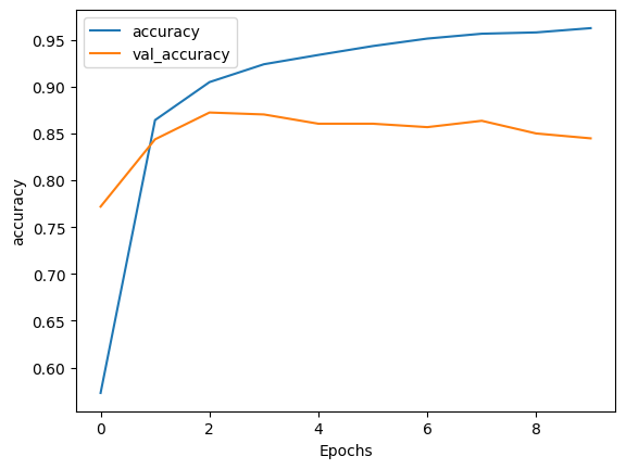
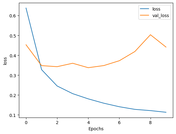
Epoch 1/10
391/391 [==============================] - 95s 231ms/step - loss: 0.6377 - accuracy: 0.5728 - val_loss: 0.4529 - val_accuracy: 0.7719
Epoch 2/10
391/391 [==============================] - 73s 186ms/step - loss: 0.3278 - accuracy: 0.8643 - val_loss: 0.3480 - val_accuracy: 0.8438
Epoch 3/10
391/391 [==============================] - 63s 160ms/step - loss: 0.2456 - accuracy: 0.9049 - val_loss: 0.3427 - val_accuracy: 0.8724
Epoch 4/10
391/391 [==============================] - 55s 139ms/step - loss: 0.2070 - accuracy: 0.9240 - val_loss: 0.3599 - val_accuracy: 0.8703
Epoch 5/10
391/391 [==============================] - 54s 136ms/step - loss: 0.1807 - accuracy: 0.9339 - val_loss: 0.3375 - val_accuracy: 0.8604
Epoch 6/10
391/391 [==============================] - 50s 126ms/step - loss: 0.1589 - accuracy: 0.9434 - val_loss: 0.3482 - val_accuracy: 0.8604
Epoch 7/10
391/391 [==============================] - 49s 124ms/step - loss: 0.1411 - accuracy: 0.9514 - val_loss: 0.3726 - val_accuracy: 0.8568
Epoch 8/10
391/391 [==============================] - 49s 123ms/step - loss: 0.1279 - accuracy: 0.9566 - val_loss: 0.4189 - val_accuracy: 0.8635
Epoch 9/10
391/391 [==============================] - 45s 115ms/step - loss: 0.1216 - accuracy: 0.9580 - val_loss: 0.5034 - val_accuracy: 0.8500
Epoch 10/10
391/391 [==============================] - 45s 113ms/step - loss: 0.1133 - accuracy: 0.9625 - val_loss: 0.4414 - val_accuracy: 0.8448
test_loss, test_acc = model.evaluate(test_dataset)

print('Test Loss: {}'.format(test_loss))
print('Test Accuracy: {}'.format(test_acc))
391/391 [==============================] - 16s 41ms/step - loss: 0.4472 - accuracy: 0.8446
Test Loss: 0.4472350776195526
Test Accuracy: 0.8445600271224976
上記のモデルはシーケンスに適用されたパディングをマスクしていません。パディングされたシーケンスで訓練を行い、パディングをしていないシーケンスでテストするとすれば、このことが結果を歪める可能性があります。理想的にはこれを避けるために、 マスキングを使うべきですが、下記のように出力への影響は小さいものでしかありません。
予測値が 0.5 以上であればポジティブ、それ以外はネガティブです。
def pad_to_size(vec, size):
  zeros = [0] * (size - len(vec))
  vec.extend(zeros)
  return vec
def sample_predict(sample_pred_text, pad):
  encoded_sample_pred_text = encoder.encode(sample_pred_text)

  if pad:
    encoded_sample_pred_text = pad_to_size(encoded_sample_pred_text, 64)
  encoded_sample_pred_text = tf.cast(encoded_sample_pred_text, tf.float32)
  predictions = model.predict(tf.expand_dims(encoded_sample_pred_text, 0))

  return (predictions)
# パディングなしのサンプルテキストの推論

sample_pred_text = ('The movie was cool. The animation and the graphics '
                    'were out of this world. I would recommend this movie.')
predictions = sample_predict(sample_pred_text, pad=False)
print(predictions)
1/1 [==============================] - 1s 655ms/step
[[-0.39028847]]
# パディングありのサンプルテキストの推論

sample_pred_text = ('The movie was cool. The animation and the graphics '
                    'were out of this world. I would recommend this movie.')
predictions = sample_predict(sample_pred_text, pad=True)
print(predictions)
1/1 [==============================] - 1s 852ms/step
[[-0.81083757]]
plot_graphs(history, 'accuracy')
plot_graphs(history, 'loss')
2つ以上の LSTM レイヤーを重ねる
Keras のリカレントレイヤーには、コンストラクタの return_sequences 引数でコントロールされる2つのモードがあります。
- それぞれのタイムステップの連続した出力のシーケンス全体(shape が
(batch_size, timesteps, output_features)の3階テンソル)を返す。 - それぞれの入力シーケンスの最後の出力だけ(shape が
(batch_size, output_features)の2階テンソル)を返す。
model = tf.keras.Sequential([
    tf.keras.layers.Embedding(encoder.vocab_size, 64),
    tf.keras.layers.Bidirectional(tf.keras.layers.LSTM(64,  return_sequences=True)),
    tf.keras.layers.Bidirectional(tf.keras.layers.LSTM(32)),
    tf.keras.layers.Dense(64, activation='relu'),
    tf.keras.layers.Dropout(0.5),
    tf.keras.layers.Dense(1)
])
model.compile(loss=tf.keras.losses.BinaryCrossentropy(from_logits=True),
              optimizer=tf.keras.optimizers.Adam(1e-4),
              metrics=['accuracy'])
history = model.fit(train_dataset, epochs=10,
                    validation_data=test_dataset,
                    validation_steps=30)
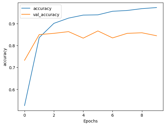
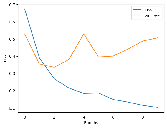
Epoch 1/10
391/391 [==============================] - 121s 293ms/step - loss: 0.6737 - accuracy: 0.5259 - val_loss: 0.5292 - val_accuracy: 0.7323
Epoch 2/10
391/391 [==============================] - 102s 259ms/step - loss: 0.3894 - accuracy: 0.8358 - val_loss: 0.3543 - val_accuracy: 0.8495
Epoch 3/10
391/391 [==============================] - 93s 236ms/step - loss: 0.2694 - accuracy: 0.9007 - val_loss: 0.3352 - val_accuracy: 0.8552
Epoch 4/10
391/391 [==============================] - 91s 231ms/step - loss: 0.2153 - accuracy: 0.9246 - val_loss: 0.3814 - val_accuracy: 0.8630
Epoch 5/10
391/391 [==============================] - 87s 221ms/step - loss: 0.1838 - accuracy: 0.9384 - val_loss: 0.5294 - val_accuracy: 0.8333
Epoch 6/10
391/391 [==============================] - 84s 213ms/step - loss: 0.1865 - accuracy: 0.9396 - val_loss: 0.3958 - val_accuracy: 0.8661
Epoch 7/10
391/391 [==============================] - 84s 214ms/step - loss: 0.1485 - accuracy: 0.9558 - val_loss: 0.4012 - val_accuracy: 0.8344
Epoch 8/10
391/391 [==============================] - 82s 209ms/step - loss: 0.1339 - accuracy: 0.9594 - val_loss: 0.4415 - val_accuracy: 0.8552
Epoch 9/10
391/391 [==============================] - 82s 209ms/step - loss: 0.1149 - accuracy: 0.9678 - val_loss: 0.4878 - val_accuracy: 0.8578
Epoch 10/10
391/391 [==============================] - 82s 209ms/step - loss: 0.1024 - accuracy: 0.9728 - val_loss: 0.5066 - val_accuracy: 0.8443
test_loss, test_acc = model.evaluate(test_dataset)

print('Test Loss: {}'.format(test_loss))
print('Test Accuracy: {}'.format(test_acc))
391/391 [==============================] - 32s 81ms/step - loss: 0.4923 - accuracy: 0.8470
Test Loss: 0.4922844171524048
Test Accuracy: 0.8470399975776672
# パディングなしのサンプルテキストの推論

sample_pred_text = ('The movie was not good. The animation and the graphics '
                    'were terrible. I would not recommend this movie.')
predictions = sample_predict(sample_pred_text, pad=False)
print(predictions)
1/1 [==============================] - 1s 1s/step
[[-2.682913]]
# パディングありのサンプルテキストの推論

sample_pred_text = ('The movie was not good. The animation and the graphics '
                    'were terrible. I would not recommend this movie.')
predictions = sample_predict(sample_pred_text, pad=True)
print(predictions)
1/1 [==============================] - 1s 1s/step
[[-3.806074]]
plot_graphs(history, 'accuracy')
plot_graphs(history, 'loss')
GRU レイヤーなど既存のほかのレイヤーを調べてみましょう。
カスタム RNN の構築に興味があるのであれば、Keras RNN ガイド を参照してください。