
| |
 GitHubでソースを表示 GitHubでソースを表示 |
このガイドでは、TensorFlow basics の簡単な概要を説明します。このドキュメントの各セクションは、より大きなトピックの概要です。各セクションの末尾に、ガイド全文へのリンクを記載しています。
TensorFlow は機械学習用のエンドツーエンドプラットフォームで、以下の内容をサポートしています。
- 多次元配列ベースの数値計算(NumPy に類似)
- GPU および分散処理
- 自動微分
- モデルの構築、トレーニング、およびエクスポート
- その他
テンソル
TensorFlow は、tf.Tensor として表現される多次元配列またはテンソルを操作します。以下は2次元テンソルです。
import tensorflow as tf

x = tf.constant([[1., 2., 3.],
                 [4., 5., 6.]])

print(x)
print(x.shape)
print(x.dtype)
2024-01-11 18:35:26.203069: E external/local_xla/xla/stream_executor/cuda/cuda_dnn.cc:9261] Unable to register cuDNN factory: Attempting to register factory for plugin cuDNN when one has already been registered
2024-01-11 18:35:26.203114: E external/local_xla/xla/stream_executor/cuda/cuda_fft.cc:607] Unable to register cuFFT factory: Attempting to register factory for plugin cuFFT when one has already been registered
2024-01-11 18:35:26.204654: E external/local_xla/xla/stream_executor/cuda/cuda_blas.cc:1515] Unable to register cuBLAS factory: Attempting to register factory for plugin cuBLAS when one has already been registered
tf.Tensor(
[[1. 2. 3.]
 [4. 5. 6.]], shape=(2, 3), dtype=float32)
(2, 3)
<dtype: 'float32'>
tf.Tensor の最も重要な属性は shape と dtype です。
Tensor.shape: 各軸に沿ったテンソルのサイズを示します。Tensor.dtype: テンソル内のすべての要素の型を示します。
TensorFlow はテンソルに標準の算術演算や機械学習に特化した多数の演算を実装します。
以下に例を示します。
x + x
<tf.Tensor: shape=(2, 3), dtype=float32, numpy=
array([[ 2.,  4.,  6.],
       [ 8., 10., 12.]], dtype=float32)>
5 * x
<tf.Tensor: shape=(2, 3), dtype=float32, numpy=
array([[ 5., 10., 15.],
       [20., 25., 30.]], dtype=float32)>
x @ tf.transpose(x)
<tf.Tensor: shape=(2, 2), dtype=float32, numpy=
array([[14., 32.],
       [32., 77.]], dtype=float32)>
tf.concat([x, x, x], axis=0)
<tf.Tensor: shape=(6, 3), dtype=float32, numpy=
array([[1., 2., 3.],
       [4., 5., 6.],
       [1., 2., 3.],
       [4., 5., 6.],
       [1., 2., 3.],
       [4., 5., 6.]], dtype=float32)>
tf.nn.softmax(x, axis=-1)
<tf.Tensor: shape=(2, 3), dtype=float32, numpy=
array([[0.09003057, 0.24472848, 0.6652409 ],
       [0.09003057, 0.24472848, 0.6652409 ]], dtype=float32)>
tf.reduce_sum(x)
<tf.Tensor: shape=(), dtype=float32, numpy=21.0>
注意: 通常、TensorFlow 関数が Tensor を入力として期待する場合、関数は tf.convert_to_tensor を使用して Tensor に変換できるものをすべて受け入れます。例については、以下を参照してください。
tf.convert_to_tensor([1,2,3])
<tf.Tensor: shape=(3,), dtype=int32, numpy=array([1, 2, 3], dtype=int32)>
tf.reduce_sum([1,2,3])
<tf.Tensor: shape=(), dtype=int32, numpy=6>
大規模な計算を CPU で実行すると低速化する可能性があります。適切に構成すれば、TensorFlow は GPU などのアクセラレータハードウェアを使用して演算を非常に素早く実行することが可能です。
if tf.config.list_physical_devices('GPU'):
  print("TensorFlow **IS** using the GPU")
else:
  print("TensorFlow **IS NOT** using the GPU")
TensorFlow **IS** using the GPU
詳細は、テンソルガイドをご覧ください。
変数
通常の tf.Tensor オブジェクトはイミュータブルです。TensorFlow にモデルの重み(またはその他のミュータブルな状態)を格納するには、tf.Variable を使用します。
var = tf.Variable([0.0, 0.0, 0.0])
var.assign([1, 2, 3])
<tf.Variable 'UnreadVariable' shape=(3,) dtype=float32, numpy=array([1., 2., 3.], dtype=float32)>
var.assign_add([1, 1, 1])
<tf.Variable 'UnreadVariable' shape=(3,) dtype=float32, numpy=array([2., 3., 4.], dtype=float32)>
詳細は、変数ガイドをご覧ください。
自動微分
最新の機械学習の基礎は、勾配降下と関連アルゴリズムです。
これを可能にするために、TensorFlow は自動微分(autodiff)を実装しており、微積分を使用して勾配を計算します。通常、モデルの重みに関する誤差または損失の勾配を計算する際にこれを使用します。
x = tf.Variable(1.0)

def f(x):
  y = x**2 + 2*x - 5
  return y
f(x)
<tf.Tensor: shape=(), dtype=float32, numpy=-2.0>
x = 1.0 の場合、y = f(x) = (1**2 + 2*1 - 5) = -2 となります。
y の導関数は y' = f'(x) = (2*x + 2) = 4 です。TensorFlow はこれを自動的に計算できます。
with tf.GradientTape() as tape:
  y = f(x)

g_x = tape.gradient(y, x)  # g(x) = dy/dx

g_x
<tf.Tensor: shape=(), dtype=float32, numpy=4.0>
この単純な例は、単一のスカラー(x)に関する導関数のみを取っていますが、TensorFlow はスカラーでない任意の数のテンソルに関する勾配を同時に計算できます。
詳細は、自動微分ガイドをご覧ください。
グラフと tf.function
TensorFlow は Python ライブラリのように対話型で使用できますが、以下を行うためのツールも提供しています。
- パフォーマンス最適化: トレーニングと推論を高速化します。
- エクスポート: モデルのトレーニングが完了したら、そのモデルを保存できます。
これらを行うには、tf.function を使用して、純粋な TensorFlow コードと Python を分離する必要があります。
@tf.function
def my_func(x):
  print('Tracing.\n')
  return tf.reduce_sum(x)
tf.function を初めて実行すると、Python として実行されますが、関数内で行われた TensorFlow 計算を表現する最適化された完全なグラフがキャプチャされます。
x = tf.constant([1, 2, 3])
my_func(x)
Tracing.
<tf.Tensor: shape=(), dtype=int32, numpy=6>
後続の呼び出しでは、TensorFlow は最適化グラフのみを実行し、TensorFlow でないステップが省略されます。以下では、my_func でトレーシングが出力されないところに注意してください。print は Python 関数であり、TensorFlow 関数ではないためです。
x = tf.constant([10, 9, 8])
my_func(x)
<tf.Tensor: shape=(), dtype=int32, numpy=27>
シグネチャ(shape と dtype)が異なる入力ではグラフを再利用できない可能性があるため、代わりに新しいグラフが生成されます。
x = tf.constant([10.0, 9.1, 8.2], dtype=tf.float32)
my_func(x)
Tracing.
<tf.Tensor: shape=(), dtype=float32, numpy=27.3>
キャプチャされたこれらのグラフには、以下の 2 つのメリットがあります。
- 多くの場合、実行速度が大幅に高速化します(このような単純な例では高速化されません)。
tf.saved_modelを使ってこれらのグラフをエクスポートすると、Python がインストールされていないサーバーやモバイルデバイスなどの他のシステムで実行することができます。
詳細は、グラフの導入をご覧ください。
モジュール、レイヤー、モデル
tf.Module は、tf.Variable オブジェクトと、それを操作する tf.function オブジェクトを管理するためのクラスです。tf.Module は、以下の重要な 2 つの機能をサポートするために必要なクラスです。
tf.train.Checkpointを使用すると、変数の値を保存し、復元することができます。モデルの状態を素早く保存して復元できるため、トレーニング中に役立ちます。tf.saved_modelを使用すると、tf.Variableの値とtf.functionグラフのインポートとエクスポートを行えます。そのため、モデルを作成した Python プログラムに頼らずに、モデルを実行することができます。
単純な tf.Module オブジェクトの完全なエクスポート例を以下に示します。
class MyModule(tf.Module):
  def __init__(self, value):
    self.weight = tf.Variable(value)

  @tf.function
  def multiply(self, x):
    return x * self.weight
mod = MyModule(3)
mod.multiply(tf.constant([1, 2, 3]))
<tf.Tensor: shape=(3,), dtype=int32, numpy=array([3, 6, 9], dtype=int32)>
Module を保存します。
save_path = './saved'
tf.saved_model.save(mod, save_path)
INFO:tensorflow:Assets written to: ./saved/assets
結果で得られる SavedModel は、それを作成したコードから独立しています。この SavedModel は、Python、その他の言語バインディング、または TensorFlow Serving から読み込むことができアンス。また、TensorFlow Lite または TensorFlow JS で実行できるように変換することも可能です。
reloaded = tf.saved_model.load(save_path)
reloaded.multiply(tf.constant([1, 2, 3]))
<tf.Tensor: shape=(3,), dtype=int32, numpy=array([3, 6, 9], dtype=int32)>
tf.keras.layers.Layer クラスと tf.keras.Model クラスは tf.Module を基礎とし、モデルを構築、トレーニング、および保存するための追加機能と便利な方法を提供します。一部の機能については、次のセクションで説明しています。
詳細は、モジュールの導入をご覧ください。
トレーニングループ
では、これらをゼロから合わせて基本的なモデルを構築し、トレーニングします。
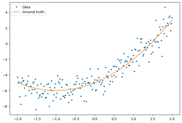
まず、サンプルデータを作成します。これは、二次曲線に緩やかに沿ったポイントクラウドを生成します。
import matplotlib
from matplotlib import pyplot as plt

matplotlib.rcParams['figure.figsize'] = [9, 6]
x = tf.linspace(-2, 2, 201)
x = tf.cast(x, tf.float32)

def f(x):
  y = x**2 + 2*x - 5
  return y

y = f(x) + tf.random.normal(shape=[201])

plt.plot(x.numpy(), y.numpy(), '.', label='Data')
plt.plot(x, f(x), label='Ground truth')
plt.legend();
ランダムに初期化した重みとバイアスを使って、二次モデルを作成します。
class Model(tf.Module):

  def __init__(self):
    # Randomly generate weight and bias terms
    rand_init = tf.random.uniform(shape=[3], minval=0., maxval=5., seed=22)
    # Initialize model parameters
    self.w_q = tf.Variable(rand_init[0])
    self.w_l = tf.Variable(rand_init[1])
    self.b = tf.Variable(rand_init[2])

  @tf.function
  def __call__(self, x):
    # Quadratic Model : quadratic_weight * x^2 + linear_weight * x + bias
    return self.w_q * (x**2) + self.w_l * x + self.b
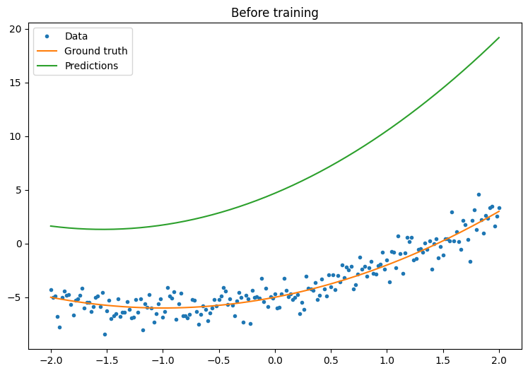
トレーニングする前に、モデルのパフォーマンスを観察します。
quad_model = Model()
def plot_preds(x, y, f, model, title):
  plt.figure()
  plt.plot(x, y, '.', label='Data')
  plt.plot(x, f(x), label='Ground truth')
  plt.plot(x, model(x), label='Predictions')
  plt.title(title)
  plt.legend()
plot_preds(x, y, f, quad_model, 'Before training')
次に、モデルtの損失を定義します。
このモデルは連続する値を予測するものであるため、損失関数には平均二乗誤差(MSE)が最適です。予測のベクトルを \(\hat{y}\) とすると、予測値とグラウンドトゥルースの二乗差の平均として定義されます。
\(MSE = \frac{1}{m}\sum_{i=1}^{m}(\hat{y}_i -y_i)^2\)
def mse_loss(y_pred, y):
  return tf.reduce_mean(tf.square(y_pred - y))
モデルの基本的なトレーニングループを記述します。このループは、モデルのパラメータを反復的に更新するために、MSE 損失関数と入力に対する勾配を利用します。トレーニングのミニバッチを使用すると、メモリ効率とより高速な収束を得られます。tf.data.Dataset API には、バッチ処理とシャッフル用の便利な関数が備わっています。
batch_size = 32
dataset = tf.data.Dataset.from_tensor_slices((x, y))
dataset = dataset.shuffle(buffer_size=x.shape[0]).batch(batch_size)
# Set training parameters
epochs = 100
learning_rate = 0.01
losses = []
# Format training loop
for epoch in range(epochs):
for x_batch, y_batch in dataset:
with tf.GradientTape() as tape:
batch_loss = mse_loss(quad_model(x_batch), y_batch)
# Update parameters with respect to the gradient calculations
grads = tape.gradient(batch_loss, quad_model.variables)
for g,v in zip(grads, quad_model.variables):
v.assign_sub(learning_rate*g)
# Keep track of model loss per epoch
loss = mse_loss(quad_model(x), y)
losses.append(loss)
if epoch % 10 == 0:
print(f'Mean squared error for step {epoch}: {loss.numpy():0.3f}')
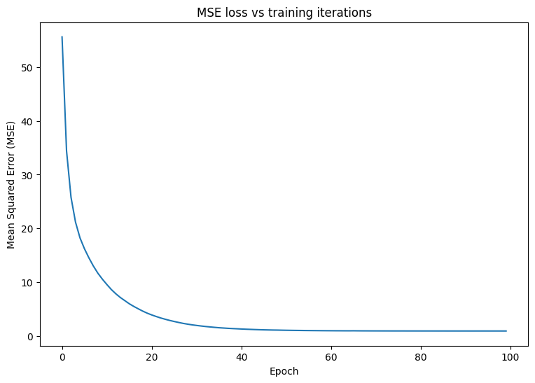
# Plot model results
print("\n")
plt.plot(range(epochs), losses)
plt.xlabel("Epoch")
plt.ylabel("Mean Squared Error (MSE)")
plt.title('MSE loss vs training iterations');
Mean squared error for step 0: 55.600
Mean squared error for step 10: 9.563
Mean squared error for step 20: 3.912
Mean squared error for step 30: 1.961
Mean squared error for step 40: 1.296
Mean squared error for step 50: 1.060
Mean squared error for step 60: 0.975
Mean squared error for step 70: 0.945
Mean squared error for step 80: 0.934
Mean squared error for step 90: 0.931
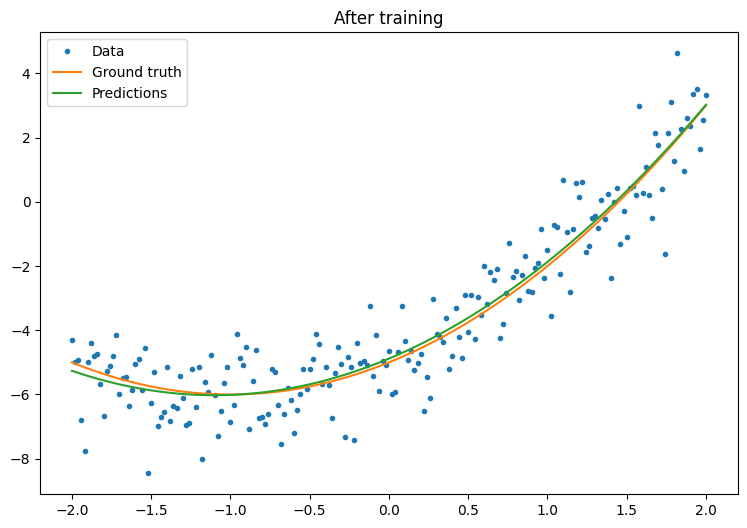
トレーニングする前に、モデルのパフォーマンスを観察しましょう。
plot_preds(x, y, f, quad_model, 'After training')
動作してはいますが、tf.keras モジュールには、共通のトレーニングユーティリティの実装が存在することを思い出してください。独自のユーティリティを記述する前に、それらを使用することを検討できます。まず、Model.compile と Model.fit メソッドを使って、トレーニングループを実装できます。
tf.keras.Sequential を使って Keras で Sequential Model を作成することから始めます。最も単純な Keras レイヤーの 1 つは Dense レイヤーです。これは、tf.keras.layers.Dense を使ってインスタンス化できます。密なレイヤーは、\(\mathrm{Y} = \mathrm{W}\mathrm{X} + \vec{b}\) の形態の多次元線形リレーションを学習できます。\(w_1x^2 + w_2x + b\) の非線形式を学習するために、密なレイヤーの入力は \(x^2\) and \(x\) を特徴量とするデータ行列である必要があります。tf.keras.layers.Lambda ラムダレイヤーは、このスタック変換を実行するために使用できます。
new_model = tf.keras.Sequential([
    tf.keras.layers.Lambda(lambda x: tf.stack([x, x**2], axis=1)),
    tf.keras.layers.Dense(units=1, kernel_initializer=tf.random.normal)])
new_model.compile(
    loss=tf.keras.losses.MSE,
    optimizer=tf.keras.optimizers.SGD(learning_rate=0.01))

history = new_model.fit(x, y,
                        epochs=100,
                        batch_size=32,
                        verbose=0)

new_model.save('./my_new_model')
WARNING: All log messages before absl::InitializeLog() is called are written to STDERR
I0000 00:00:1704998137.631935   85850 device_compiler.h:186] Compiled cluster using XLA!  This line is logged at most once for the lifetime of the process.
INFO:tensorflow:Unsupported signature for serialization: ((TensorSpec(shape=(2, 1), dtype=tf.float32, name='gradient'), <tensorflow.python.framework.func_graph.UnknownArgument object at 0x7fc26c6e00a0>, 140473019619168), {}).
INFO:tensorflow:Unsupported signature for serialization: ((TensorSpec(shape=(2, 1), dtype=tf.float32, name='gradient'), <tensorflow.python.framework.func_graph.UnknownArgument object at 0x7fc26c6e00a0>, 140473019619168), {}).
INFO:tensorflow:Unsupported signature for serialization: ((TensorSpec(shape=(1,), dtype=tf.float32, name='gradient'), <tensorflow.python.framework.func_graph.UnknownArgument object at 0x7fc26c60afd0>, 140473019125312), {}).
INFO:tensorflow:Unsupported signature for serialization: ((TensorSpec(shape=(1,), dtype=tf.float32, name='gradient'), <tensorflow.python.framework.func_graph.UnknownArgument object at 0x7fc26c60afd0>, 140473019125312), {}).
INFO:tensorflow:Unsupported signature for serialization: ((TensorSpec(shape=(2, 1), dtype=tf.float32, name='gradient'), <tensorflow.python.framework.func_graph.UnknownArgument object at 0x7fc26c6e00a0>, 140473019619168), {}).
INFO:tensorflow:Unsupported signature for serialization: ((TensorSpec(shape=(2, 1), dtype=tf.float32, name='gradient'), <tensorflow.python.framework.func_graph.UnknownArgument object at 0x7fc26c6e00a0>, 140473019619168), {}).
INFO:tensorflow:Unsupported signature for serialization: ((TensorSpec(shape=(1,), dtype=tf.float32, name='gradient'), <tensorflow.python.framework.func_graph.UnknownArgument object at 0x7fc26c60afd0>, 140473019125312), {}).
INFO:tensorflow:Unsupported signature for serialization: ((TensorSpec(shape=(1,), dtype=tf.float32, name='gradient'), <tensorflow.python.framework.func_graph.UnknownArgument object at 0x7fc26c60afd0>, 140473019125312), {}).
INFO:tensorflow:Assets written to: ./my_new_model/assets
INFO:tensorflow:Assets written to: ./my_new_model/assets
/tmpfs/src/tf_docs_env/lib/python3.9/site-packages/keras/src/initializers/__init__.py:144: UserWarning: The `keras.initializers.serialize()` API should only be used for objects of type `keras.initializers.Initializer`. Found an instance of type <class 'function'>, which may lead to improper serialization.
  warnings.warn(
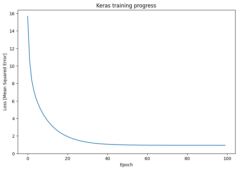
トレーニング後の Keras モデルのパフォーマンスを観察します。
plt.plot(history.history['loss'])
plt.xlabel('Epoch')
plt.ylim([0, max(plt.ylim())])
plt.ylabel('Loss [Mean Squared Error]')
plt.title('Keras training progress');
plot_preds(x, y, f, new_model, 'After Training: Keras')
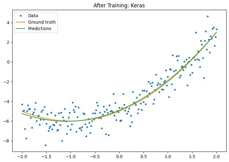
詳細は、基本トレーニングループと Keras ガイドをご覧ください。