
| | |  Ver no GitHub Ver no GitHub | | |
Este filme classifica notebook opiniões como positivo ou negativo usando o texto da revisão. Este é um exemplo de binário de duas classes-classificação -ou, um tipo importante e amplamente aplicáveis de problema de aprendizagem de máquina.
Nós vamos usar o dataset IMDB que contém o texto de 50.000 revisões de filme da Internet Movie Database . Elas são divididas em 25.000 análises para treinamento e 25.000 análises para teste. Os conjuntos de treinamento e teste são equilibradas, o que significa que contêm o mesmo número de comentários positivos e negativos.
Este notebook usa tf.keras , uma API de alto nível para modelos de construção e de trem em TensorFlow e TensorFlow Hub , uma biblioteca e uma plataforma para a aprendizagem de transferência. Para um texto mais avançado de classificação tutorial usando tf.keras , consulte o MLCC texto Guia de Classificação .
Mais modelos
Aqui você pode encontrar modelos mais expressivas ou de elevada performance que você pode usar para gerar a incorporação de texto.
Configurar
import numpy as np

import tensorflow as tf
import tensorflow_hub as hub
import tensorflow_datasets as tfds

import matplotlib.pyplot as plt

print("Version: ", tf.__version__)
print("Eager mode: ", tf.executing_eagerly())
print("Hub version: ", hub.__version__)
print("GPU is", "available" if tf.config.list_physical_devices('GPU') else "NOT AVAILABLE")
Version:  2.7.0
Eager mode:  True
Hub version:  0.12.0
GPU is available
Baixe o conjunto de dados IMDB
O conjunto de dados IMDB está disponível em conjuntos de dados TensorFlow . O código a seguir baixa o conjunto de dados IMDB para sua máquina (ou o tempo de execução colab):
train_data, test_data = tfds.load(name="imdb_reviews", split=["train", "test"],
                                  batch_size=-1, as_supervised=True)

train_examples, train_labels = tfds.as_numpy(train_data)
test_examples, test_labels = tfds.as_numpy(test_data)
WARNING:tensorflow:From /tmpfs/src/tf_docs_env/lib/python3.7/site-packages/tensorflow_datasets/core/dataset_builder.py:622: get_single_element (from tensorflow.python.data.experimental.ops.get_single_element) is deprecated and will be removed in a future version.
Instructions for updating:
Use `tf.data.Dataset.get_single_element()`.
Explore os dados
Vamos dedicar um momento para entender o formato dos dados. Cada exemplo é uma frase que representa a crítica do filme e um rótulo correspondente. A frase não é pré-processada de forma alguma. O rótulo é um valor inteiro de 0 ou 1, em que 0 é uma resenha negativa e 1 é uma resenha positiva.
print("Training entries: {}, test entries: {}".format(len(train_examples), len(test_examples)))
Training entries: 25000, test entries: 25000
Vamos imprimir os primeiros 10 exemplos.
train_examples[:10]
array([b"This was an absolutely terrible movie. Don't be lured in by Christopher Walken or Michael Ironside. Both are great actors, but this must simply be their worst role in history. Even their great acting could not redeem this movie's ridiculous storyline. This movie is an early nineties US propaganda piece. The most pathetic scenes were those when the Columbian rebels were making their cases for revolutions. Maria Conchita Alonso appeared phony, and her pseudo-love affair with Walken was nothing but a pathetic emotional plug in a movie that was devoid of any real meaning. I am disappointed that there are movies like this, ruining actor's like Christopher Walken's good name. I could barely sit through it.",
       b'I have been known to fall asleep during films, but this is usually due to a combination of things including, really tired, being warm and comfortable on the sette and having just eaten a lot. However on this occasion I fell asleep because the film was rubbish. The plot development was constant. Constantly slow and boring. Things seemed to happen, but with no explanation of what was causing them or why. I admit, I may have missed part of the film, but i watched the majority of it and everything just seemed to happen of its own accord without any real concern for anything else. I cant recommend this film at all.',
       b'Mann photographs the Alberta Rocky Mountains in a superb fashion, and Jimmy Stewart and Walter Brennan give enjoyable performances as they always seem to do. <br /><br />But come on Hollywood - a Mountie telling the people of Dawson City, Yukon to elect themselves a marshal (yes a marshal!) and to enforce the law themselves, then gunfighters battling it out on the streets for control of the town? <br /><br />Nothing even remotely resembling that happened on the Canadian side of the border during the Klondike gold rush. Mr. Mann and company appear to have mistaken Dawson City for Deadwood, the Canadian North for the American Wild West.<br /><br />Canadian viewers be prepared for a Reefer Madness type of enjoyable howl with this ludicrous plot, or, to shake your head in disgust.',
       b'This is the kind of film for a snowy Sunday afternoon when the rest of the world can go ahead with its own business as you descend into a big arm-chair and mellow for a couple of hours. Wonderful performances from Cher and Nicolas Cage (as always) gently row the plot along. There are no rapids to cross, no dangerous waters, just a warm and witty paddle through New York life at its best. A family film in every sense and one that deserves the praise it received.',
       b'As others have mentioned, all the women that go nude in this film are mostly absolutely gorgeous. The plot very ably shows the hypocrisy of the female libido. When men are around they want to be pursued, but when no "men" are around, they become the pursuers of a 14 year old boy. And the boy becomes a man really fast (we should all be so lucky at this age!). He then gets up the courage to pursue his true love.',
       b"This is a film which should be seen by anybody interested in, effected by, or suffering from an eating disorder. It is an amazingly accurate and sensitive portrayal of bulimia in a teenage girl, its causes and its symptoms. The girl is played by one of the most brilliant young actresses working in cinema today, Alison Lohman, who was later so spectacular in 'Where the Truth Lies'. I would recommend that this film be shown in all schools, as you will never see a better on this subject. Alison Lohman is absolutely outstanding, and one marvels at her ability to convey the anguish of a girl suffering from this compulsive disorder. If barometers tell us the air pressure, Alison Lohman tells us the emotional pressure with the same degree of accuracy. Her emotional range is so precise, each scene could be measured microscopically for its gradations of trauma, on a scale of rising hysteria and desperation which reaches unbearable intensity. Mare Winningham is the perfect choice to play her mother, and does so with immense sympathy and a range of emotions just as finely tuned as Lohman's. Together, they make a pair of sensitive emotional oscillators vibrating in resonance with one another. This film is really an astonishing achievement, and director Katt Shea should be proud of it. The only reason for not seeing it is if you are not interested in people. But even if you like nature films best, this is after all animal behaviour at the sharp edge. Bulimia is an extreme version of how a tormented soul can destroy her own body in a frenzy of despair. And if we don't sympathise with people suffering from the depths of despair, then we are dead inside.",
       b'Okay, you have:<br /><br />Penelope Keith as Miss Herringbone-Tweed, B.B.E. (Backbone of England.) She\'s killed off in the first scene - that\'s right, folks; this show has no backbone!<br /><br />Peter O\'Toole as Ol\' Colonel Cricket from The First War and now the emblazered Lord of the Manor.<br /><br />Joanna Lumley as the ensweatered Lady of the Manor, 20 years younger than the colonel and 20 years past her own prime but still glamourous (Brit spelling, not mine) enough to have a toy-boy on the side. It\'s alright, they have Col. Cricket\'s full knowledge and consent (they guy even comes \'round for Christmas!) Still, she\'s considerate of the colonel enough to have said toy-boy her own age (what a gal!)<br /><br />David McCallum as said toy-boy, equally as pointlessly glamourous as his squeeze. Pilcher couldn\'t come up with any cover for him within the story, so she gave him a hush-hush job at the Circus.<br /><br />and finally:<br /><br />Susan Hampshire as Miss Polonia Teacups, Venerable Headmistress of the Venerable Girls\' Boarding-School, serving tea in her office with a dash of deep, poignant advice for life in the outside world just before graduation. Her best bit of advice: "I\'ve only been to Nancherrow (the local Stately Home of England) once. I thought it was very beautiful but, somehow, not part of the real world." Well, we can\'t say they didn\'t warn us.<br /><br />Ah, Susan - time was, your character would have been running the whole show. They don\'t write \'em like that any more. Our loss, not yours.<br /><br />So - with a cast and setting like this, you have the re-makings of "Brideshead Revisited," right?<br /><br />Wrong! They took these 1-dimensional supporting roles because they paid so well. After all, acting is one of the oldest temp-jobs there is (YOU name another!)<br /><br />First warning sign: lots and lots of backlighting. They get around it by shooting outdoors - "hey, it\'s just the sunlight!"<br /><br />Second warning sign: Leading Lady cries a lot. When not crying, her eyes are moist. That\'s the law of romance novels: Leading Lady is "dewy-eyed."<br /><br />Henceforth, Leading Lady shall be known as L.L.<br /><br />Third warning sign: L.L. actually has stars in her eyes when she\'s in love. Still, I\'ll give Emily Mortimer an award just for having to act with that spotlight in her eyes (I wonder . did they use contacts?)<br /><br />And lastly, fourth warning sign: no on-screen female character is "Mrs." She\'s either "Miss" or "Lady."<br /><br />When all was said and done, I still couldn\'t tell you who was pursuing whom and why. I couldn\'t even tell you what was said and done.<br /><br />To sum up: they all live through World War II without anything happening to them at all.<br /><br />OK, at the end, L.L. finds she\'s lost her parents to the Japanese prison camps and baby sis comes home catatonic. Meanwhile (there\'s always a "meanwhile,") some young guy L.L. had a crush on (when, I don\'t know) comes home from some wartime tough spot and is found living on the street by Lady of the Manor (must be some street if SHE\'s going to find him there.) Both war casualties are whisked away to recover at Nancherrow (SOMEBODY has to be "whisked away" SOMEWHERE in these romance stories!)<br /><br />Great drama.',
       b'The film is based on a genuine 1950s novel.<br /><br />Journalist Colin McInnes wrote a set of three "London novels": "Absolute Beginners", "City of Spades" and "Mr Love and Justice". I have read all three. The first two are excellent. The last, perhaps an experiment that did not come off. But McInnes\'s work is highly acclaimed; and rightly so. This musical is the novelist\'s ultimate nightmare - to see the fruits of one\'s mind being turned into a glitzy, badly-acted, soporific one-dimensional apology of a film that says it captures the spirit of 1950s London, and does nothing of the sort.<br /><br />Thank goodness Colin McInnes wasn\'t alive to witness it.',
       b'I really love the sexy action and sci-fi films of the sixties and its because of the actress\'s that appeared in them. They found the sexiest women to be in these films and it didn\'t matter if they could act (Remember "Candy"?). The reason I was disappointed by this film was because it wasn\'t nostalgic enough. The story here has a European sci-fi film called "Dragonfly" being made and the director is fired. So the producers decide to let a young aspiring filmmaker (Jeremy Davies) to complete the picture. They\'re is one real beautiful woman in the film who plays Dragonfly but she\'s barely in it. Film is written and directed by Roman Coppola who uses some of his fathers exploits from his early days and puts it into the script. I wish the film could have been an homage to those early films. They could have lots of cameos by actors who appeared in them. There is one actor in this film who was popular from the sixties and its John Phillip Law (Barbarella). Gerard Depardieu, Giancarlo Giannini and Dean Stockwell appear as well. I guess I\'m going to have to continue waiting for a director to make a good homage to the films of the sixties. If any are reading this, "Make it as sexy as you can"! I\'ll be waiting!',
       b'Sure, this one isn\'t really a blockbuster, nor does it target such a position. "Dieter" is the first name of a quite popular German musician, who is either loved or hated for his kind of acting and thats exactly what this movie is about. It is based on the autobiography "Dieter Bohlen" wrote a few years ago but isn\'t meant to be accurate on that. The movie is filled with some sexual offensive content (at least for American standard) which is either amusing (not for the other "actors" of course) or dumb - it depends on your individual kind of humor or on you being a "Bohlen"-Fan or not. Technically speaking there isn\'t much to criticize. Speaking of me I find this movie to be an OK-movie.'],
      dtype=object)
Vamos também imprimir as primeiras 10 etiquetas.
train_labels[:10]
array([0, 0, 0, 1, 1, 1, 0, 0, 0, 0])
Construir o modelo
A rede neural é criada empilhando camadas - isso requer três decisões arquitetônicas principais:
- Como representar o texto?
- Quantas camadas usar no modelo?
- Quantas unidades escondido para usar para cada camada?
Neste exemplo, os dados de entrada consistem em sentenças. Os rótulos a prever são 0 ou 1.
Uma forma de representar o texto é converter frases em vetores de embeddings. Podemos usar uma incorporação de texto pré-treinada como a primeira camada, o que terá duas vantagens:
- não precisamos nos preocupar com o pré-processamento de texto,
- podemos nos beneficiar da aprendizagem por transferência.
Para este exemplo, vamos utilizar um modelo de TensorFlow Hub chamado google / nnlm-en-dim50 / 2 .
Existem dois outros modelos para testar neste tutorial:
- google / nnlm-en-dim50-com-a normalização / 2 - mesmo que google / nnlm-en-dim50 / 2 , mas com normalização texto adicional para remover a pontuação. Isso pode ajudar a obter uma melhor cobertura de embeddings no vocabulário para tokens em seu texto de entrada.
- Google / nnlm-en-dim128-com-normalização / 2 - Um modelo maior, com uma dimensão de imersão de 128 em vez do menor 50.
Vamos primeiro criar uma camada Keras que usa um modelo TensorFlow Hub para incorporar as frases e testá-la em alguns exemplos de entrada. Note-se que a forma das incorporações produzidos saída é um esperado: (num_examples, embedding_dimension) .
model = "https://tfhub.dev/google/nnlm-en-dim50/2"
hub_layer = hub.KerasLayer(model, input_shape=[], dtype=tf.string, trainable=True)
hub_layer(train_examples[:3])
<tf.Tensor: shape=(3, 50), dtype=float32, numpy=
array([[ 0.5423194 , -0.01190171,  0.06337537,  0.0686297 , -0.16776839,
        -0.10581177,  0.168653  , -0.04998823, -0.31148052,  0.07910344,
         0.15442258,  0.01488661,  0.03930155,  0.19772716, -0.12215477,
        -0.04120982, -0.27041087, -0.21922147,  0.26517656, -0.80739075,
         0.25833526, -0.31004202,  0.2868321 ,  0.19433866, -0.29036498,
         0.0386285 , -0.78444123, -0.04793238,  0.41102988, -0.36388886,
        -0.58034706,  0.30269453,  0.36308962, -0.15227163, -0.4439151 ,
         0.19462997,  0.19528405,  0.05666233,  0.2890704 , -0.28468323,
        -0.00531206,  0.0571938 , -0.3201319 , -0.04418665, -0.08550781,
        -0.55847436, -0.2333639 , -0.20782956, -0.03543065, -0.17533456],
       [ 0.56338924, -0.12339553, -0.10862677,  0.7753425 , -0.07667087,
        -0.15752274,  0.01872334, -0.08169781, -0.3521876 ,  0.46373403,
        -0.08492758,  0.07166861, -0.00670818,  0.12686071, -0.19326551,
        -0.5262643 , -0.32958236,  0.14394784,  0.09043556, -0.54175544,
         0.02468163, -0.15456744,  0.68333143,  0.09068333, -0.45327246,
         0.23180094, -0.8615696 ,  0.3448039 ,  0.12838459, -0.58759046,
        -0.40712303,  0.23061076,  0.48426905, -0.2712814 , -0.5380918 ,
         0.47016335,  0.2257274 , -0.00830665,  0.28462422, -0.30498496,
         0.04400366,  0.25025868,  0.14867125,  0.4071703 , -0.15422425,
        -0.06878027, -0.40825695, -0.31492147,  0.09283663, -0.20183429],
       [ 0.7456156 ,  0.21256858,  0.1440033 ,  0.52338624,  0.11032254,
         0.00902788, -0.36678016, -0.08938274, -0.24165548,  0.33384597,
        -0.111946  , -0.01460045, -0.00716449,  0.19562715,  0.00685217,
        -0.24886714, -0.42796353,  0.1862    , -0.05241097, -0.664625  ,
         0.13449019, -0.22205493,  0.08633009,  0.43685383,  0.2972681 ,
         0.36140728, -0.71968895,  0.05291242, -0.1431612 , -0.15733941,
        -0.15056324, -0.05988007, -0.08178931, -0.15569413, -0.09303784,
        -0.18971168,  0.0762079 , -0.02541647, -0.27134502, -0.3392682 ,
        -0.10296471, -0.27275252, -0.34078008,  0.20083308, -0.26644838,
         0.00655449, -0.05141485, -0.04261916, -0.4541363 ,  0.20023566]],
      dtype=float32)>
Vamos agora construir o modelo completo:
model = tf.keras.Sequential()
model.add(hub_layer)
model.add(tf.keras.layers.Dense(16, activation='relu'))
model.add(tf.keras.layers.Dense(1))

model.summary()
Model: "sequential"
_________________________________________________________________
 Layer (type)                Output Shape              Param #
=================================================================
 keras_layer (KerasLayer)    (None, 50)                48190600

 dense (Dense)               (None, 16)                816

 dense_1 (Dense)             (None, 1)                 17

=================================================================
Total params: 48,191,433
Trainable params: 48,191,433
Non-trainable params: 0
_________________________________________________________________
As camadas são empilhadas sequencialmente para construir o classificador:
- A primeira camada é uma camada TensorFlow Hub. Esta camada usa um modelo salvo pré-treinado para mapear uma frase em seu vetor de incorporação. O modelo que estamos a utilizar ( google / nnlm-en-dim50 / 2 ) divide a frase em tokens, incorpora cada sinal e, em seguida, combina o de incorporação. As dimensões resultantes são:
(num_examples, embedding_dimension). - Este vector de saída de comprimento fixo é canalizada através de uma totalmente ligado (
Densecamada) com 16 unidades escondidos. - A última camada está densamente conectada a um único nó de saída. Isso gera logits: o log-odds da verdadeira classe, de acordo com o modelo.
Unidades ocultas
O modelo acima possui duas camadas intermediárias ou "ocultas", entre a entrada e a saída. O número de saídas (unidades, nós ou neurônios) é a dimensão do espaço representacional para a camada. Em outras palavras, a quantidade de liberdade que a rede tem ao aprender uma representação interna.
Se um modelo tiver mais unidades ocultas (um espaço de representação de dimensão superior) e / ou mais camadas, a rede pode aprender representações mais complexas. No entanto, torna a rede mais cara computacionalmente e pode levar ao aprendizado de padrões indesejados - padrões que melhoram o desempenho nos dados de treinamento, mas não nos dados de teste. Isso é chamado overfitting, e vamos explorar isso mais tarde.
Função de perda e otimizador
Um modelo precisa de uma função de perda e um otimizador para treinamento. Uma vez que este é um problema de classificação binária eo modelo de saídas uma probabilidade (a camada única unidade com um ativação sigmóide), usaremos o binary_crossentropy função de perda.
Esta não é a única escolha para uma função de perda, você poderia, por exemplo, escolher mean_squared_error . Mas, geralmente, binary_crossentropy é melhor para lidar com probabilidades-lo mede a "distância" entre distribuições de probabilidade, ou no nosso caso, entre a distribuição terra-verdade e as previsões.
Mais tarde, quando estivermos explorando problemas de regressão (digamos, para prever o preço de uma casa), veremos como usar outra função de perda chamada erro quadrático médio.
Agora, configure o modelo para usar um otimizador e uma função de perda:
model.compile(optimizer='adam',
              loss=tf.losses.BinaryCrossentropy(from_logits=True),
              metrics=[tf.metrics.BinaryAccuracy(threshold=0.0, name='accuracy')])
Crie um conjunto de validação
Ao treinar, queremos verificar a precisão do modelo em dados que não vimos antes. Criar um conjunto de validação, definindo além de 10.000 exemplos a partir dos dados de treinamento originais. (Por que não usar o conjunto de teste agora? Nosso objetivo é desenvolver e ajustar nosso modelo usando apenas os dados de treinamento e, em seguida, usar os dados de teste apenas uma vez para avaliar nossa precisão).
x_val = train_examples[:10000]
partial_x_train = train_examples[10000:]

y_val = train_labels[:10000]
partial_y_train = train_labels[10000:]
Treine o modelo
Treine o modelo por 40 épocas em minilotes de 512 amostras. Esta é de 40 iterações sobre todas as amostras nas x_train e y_train tensores. Durante o treinamento, monitore a perda e a precisão do modelo nas 10.000 amostras do conjunto de validação:
history = model.fit(partial_x_train,
                    partial_y_train,
                    epochs=40,
                    batch_size=512,
                    validation_data=(x_val, y_val),
                    verbose=1)
Epoch 1/40
30/30 [==============================] - 2s 34ms/step - loss: 0.6667 - accuracy: 0.6060 - val_loss: 0.6192 - val_accuracy: 0.7195
Epoch 2/40
30/30 [==============================] - 1s 28ms/step - loss: 0.5609 - accuracy: 0.7770 - val_loss: 0.5155 - val_accuracy: 0.7882
Epoch 3/40
30/30 [==============================] - 1s 29ms/step - loss: 0.4309 - accuracy: 0.8489 - val_loss: 0.4135 - val_accuracy: 0.8364
Epoch 4/40
30/30 [==============================] - 1s 28ms/step - loss: 0.3154 - accuracy: 0.8937 - val_loss: 0.3515 - val_accuracy: 0.8583
Epoch 5/40
30/30 [==============================] - 1s 29ms/step - loss: 0.2345 - accuracy: 0.9227 - val_loss: 0.3256 - val_accuracy: 0.8639
Epoch 6/40
30/30 [==============================] - 1s 28ms/step - loss: 0.1773 - accuracy: 0.9457 - val_loss: 0.3104 - val_accuracy: 0.8702
Epoch 7/40
30/30 [==============================] - 1s 29ms/step - loss: 0.1331 - accuracy: 0.9645 - val_loss: 0.3024 - val_accuracy: 0.8741
Epoch 8/40
30/30 [==============================] - 1s 28ms/step - loss: 0.0984 - accuracy: 0.9777 - val_loss: 0.3061 - val_accuracy: 0.8758
Epoch 9/40
30/30 [==============================] - 1s 29ms/step - loss: 0.0707 - accuracy: 0.9869 - val_loss: 0.3136 - val_accuracy: 0.8745
Epoch 10/40
30/30 [==============================] - 1s 29ms/step - loss: 0.0501 - accuracy: 0.9919 - val_loss: 0.3305 - val_accuracy: 0.8743
Epoch 11/40
30/30 [==============================] - 1s 28ms/step - loss: 0.0351 - accuracy: 0.9960 - val_loss: 0.3434 - val_accuracy: 0.8726
Epoch 12/40
30/30 [==============================] - 1s 29ms/step - loss: 0.0247 - accuracy: 0.9984 - val_loss: 0.3568 - val_accuracy: 0.8722
Epoch 13/40
30/30 [==============================] - 1s 29ms/step - loss: 0.0178 - accuracy: 0.9993 - val_loss: 0.3711 - val_accuracy: 0.8700
Epoch 14/40
30/30 [==============================] - 1s 30ms/step - loss: 0.0134 - accuracy: 0.9996 - val_loss: 0.3839 - val_accuracy: 0.8711
Epoch 15/40
30/30 [==============================] - 1s 29ms/step - loss: 0.0103 - accuracy: 0.9998 - val_loss: 0.3968 - val_accuracy: 0.8701
Epoch 16/40
30/30 [==============================] - 1s 29ms/step - loss: 0.0080 - accuracy: 0.9998 - val_loss: 0.4104 - val_accuracy: 0.8702
Epoch 17/40
30/30 [==============================] - 1s 29ms/step - loss: 0.0063 - accuracy: 0.9999 - val_loss: 0.4199 - val_accuracy: 0.8694
Epoch 18/40
30/30 [==============================] - 1s 28ms/step - loss: 0.0051 - accuracy: 1.0000 - val_loss: 0.4305 - val_accuracy: 0.8691
Epoch 19/40
30/30 [==============================] - 1s 28ms/step - loss: 0.0043 - accuracy: 1.0000 - val_loss: 0.4403 - val_accuracy: 0.8688
Epoch 20/40
30/30 [==============================] - 1s 29ms/step - loss: 0.0036 - accuracy: 1.0000 - val_loss: 0.4493 - val_accuracy: 0.8687
Epoch 21/40
30/30 [==============================] - 1s 30ms/step - loss: 0.0031 - accuracy: 1.0000 - val_loss: 0.4580 - val_accuracy: 0.8682
Epoch 22/40
30/30 [==============================] - 1s 30ms/step - loss: 0.0027 - accuracy: 1.0000 - val_loss: 0.4659 - val_accuracy: 0.8682
Epoch 23/40
30/30 [==============================] - 1s 31ms/step - loss: 0.0023 - accuracy: 1.0000 - val_loss: 0.4743 - val_accuracy: 0.8680
Epoch 24/40
30/30 [==============================] - 1s 29ms/step - loss: 0.0020 - accuracy: 1.0000 - val_loss: 0.4808 - val_accuracy: 0.8678
Epoch 25/40
30/30 [==============================] - 1s 30ms/step - loss: 0.0018 - accuracy: 1.0000 - val_loss: 0.4879 - val_accuracy: 0.8669
Epoch 26/40
30/30 [==============================] - 1s 30ms/step - loss: 0.0016 - accuracy: 1.0000 - val_loss: 0.4943 - val_accuracy: 0.8667
Epoch 27/40
30/30 [==============================] - 1s 29ms/step - loss: 0.0015 - accuracy: 1.0000 - val_loss: 0.5003 - val_accuracy: 0.8672
Epoch 28/40
30/30 [==============================] - 1s 29ms/step - loss: 0.0013 - accuracy: 1.0000 - val_loss: 0.5064 - val_accuracy: 0.8665
Epoch 29/40
30/30 [==============================] - 1s 29ms/step - loss: 0.0012 - accuracy: 1.0000 - val_loss: 0.5120 - val_accuracy: 0.8668
Epoch 30/40
30/30 [==============================] - 1s 30ms/step - loss: 0.0011 - accuracy: 1.0000 - val_loss: 0.5174 - val_accuracy: 0.8671
Epoch 31/40
30/30 [==============================] - 1s 30ms/step - loss: 0.0010 - accuracy: 1.0000 - val_loss: 0.5230 - val_accuracy: 0.8664
Epoch 32/40
30/30 [==============================] - 1s 29ms/step - loss: 9.2117e-04 - accuracy: 1.0000 - val_loss: 0.5281 - val_accuracy: 0.8663
Epoch 33/40
30/30 [==============================] - 1s 29ms/step - loss: 8.4693e-04 - accuracy: 1.0000 - val_loss: 0.5332 - val_accuracy: 0.8659
Epoch 34/40
30/30 [==============================] - 1s 30ms/step - loss: 7.8501e-04 - accuracy: 1.0000 - val_loss: 0.5376 - val_accuracy: 0.8666
Epoch 35/40
30/30 [==============================] - 1s 29ms/step - loss: 7.2613e-04 - accuracy: 1.0000 - val_loss: 0.5424 - val_accuracy: 0.8657
Epoch 36/40
30/30 [==============================] - 1s 29ms/step - loss: 6.7541e-04 - accuracy: 1.0000 - val_loss: 0.5468 - val_accuracy: 0.8659
Epoch 37/40
30/30 [==============================] - 1s 29ms/step - loss: 6.2841e-04 - accuracy: 1.0000 - val_loss: 0.5510 - val_accuracy: 0.8658
Epoch 38/40
30/30 [==============================] - 1s 29ms/step - loss: 5.8661e-04 - accuracy: 1.0000 - val_loss: 0.5553 - val_accuracy: 0.8656
Epoch 39/40
30/30 [==============================] - 1s 29ms/step - loss: 5.4869e-04 - accuracy: 1.0000 - val_loss: 0.5595 - val_accuracy: 0.8658
Epoch 40/40
30/30 [==============================] - 1s 30ms/step - loss: 5.1370e-04 - accuracy: 1.0000 - val_loss: 0.5635 - val_accuracy: 0.8659
Avalie o modelo
E vamos ver como o modelo funciona. Dois valores serão retornados. Perda (um número que representa nosso erro, valores mais baixos são melhores) e precisão.
results = model.evaluate(test_examples, test_labels)

print(results)
782/782 [==============================] - 2s 3ms/step - loss: 0.6272 - accuracy: 0.8484
[0.6272369027137756, 0.848360002040863]
Essa abordagem bastante ingênua atinge uma precisão de cerca de 87%. Com abordagens mais avançadas, o modelo deve se aproximar de 95%.
Crie um gráfico de precisão e perda ao longo do tempo
model.fit() retorna uma History objeto que contém um dicionário com tudo o que aconteceu durante o treinamento:
history_dict = history.history
history_dict.keys()
dict_keys(['loss', 'accuracy', 'val_loss', 'val_accuracy'])
Existem quatro entradas: uma para cada métrica monitorada durante o treinamento e a validação. Podemos usá-los para traçar a perda de treinamento e validação para comparação, bem como a precisão do treinamento e da validação:
acc = history_dict['accuracy']
val_acc = history_dict['val_accuracy']
loss = history_dict['loss']
val_loss = history_dict['val_loss']
epochs = range(1, len(acc) + 1)
# "bo" is for "blue dot"
plt.plot(epochs, loss, 'bo', label='Training loss')
# b is for "solid blue line"
plt.plot(epochs, val_loss, 'b', label='Validation loss')
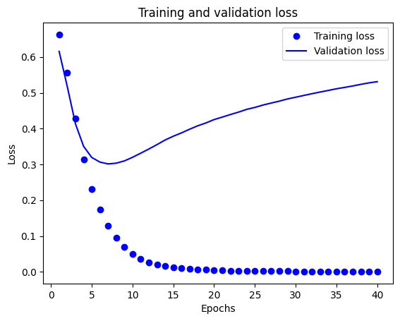
plt.title('Training and validation loss')
plt.xlabel('Epochs')
plt.ylabel('Loss')
plt.legend()
plt.show()
plt.clf()   # clear figure

plt.plot(epochs, acc, 'bo', label='Training acc')
plt.plot(epochs, val_acc, 'b', label='Validation acc')
plt.title('Training and validation accuracy')
plt.xlabel('Epochs')
plt.ylabel('Accuracy')
plt.legend()

plt.show()
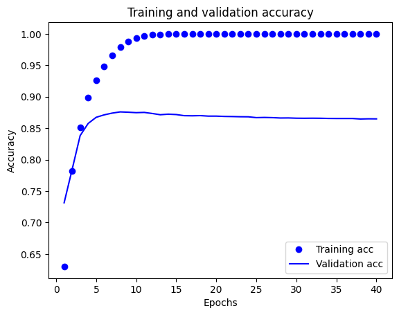
Neste gráfico, os pontos representam a perda e a precisão do treinamento, e as linhas sólidas são a perda e a precisão da validação.
Observe a perda de formação diminui com cada época ea precisão de treinamento aumenta com cada época. Isso é esperado ao usar uma otimização de gradiente descendente - deve minimizar a quantidade desejada em cada iteração.
Este não é o caso da perda de validação e precisão - eles parecem atingir o pico depois de cerca de vinte épocas. Este é um exemplo de sobreajuste: o modelo tem um desempenho melhor nos dados de treinamento do que nos dados que nunca viu antes. Após este ponto, o modelo mais-otimiza e aprende representações específicas para os dados de treinamento que não generalizam para dados de teste.
Para este caso específico, poderíamos evitar o sobreajuste simplesmente interrompendo o treinamento após cerca de vinte épocas. Posteriormente, você verá como fazer isso automaticamente com um retorno de chamada.
# MIT License
#
# Copyright (c) 2017 François Chollet
#
# Permission is hereby granted, free of charge, to any person obtaining a
# copy of this software and associated documentation files (the "Software"),
# to deal in the Software without restriction, including without limitation
# the rights to use, copy, modify, merge, publish, distribute, sublicense,
# and/or sell copies of the Software, and to permit persons to whom the
# Software is furnished to do so, subject to the following conditions:
#
# The above copyright notice and this permission notice shall be included in
# all copies or substantial portions of the Software.
#
# THE SOFTWARE IS PROVIDED "AS IS", WITHOUT WARRANTY OF ANY KIND, EXPRESS OR
# IMPLIED, INCLUDING BUT NOT LIMITED TO THE WARRANTIES OF MERCHANTABILITY,
# FITNESS FOR A PARTICULAR PURPOSE AND NONINFRINGEMENT. IN NO EVENT SHALL
# THE AUTHORS OR COPYRIGHT HOLDERS BE LIABLE FOR ANY CLAIM, DAMAGES OR OTHER
# LIABILITY, WHETHER IN AN ACTION OF CONTRACT, TORT OR OTHERWISE, ARISING
# FROM, OUT OF OR IN CONNECTION WITH THE SOFTWARE OR THE USE OR OTHER
# DEALINGS IN THE SOFTWARE.