
| | |  GitHub에서 소스 보기 GitHub에서 소스 보기 | |
설정
먼저 이 데모에 사용된 패키지를 설치합니다.
pip install -q dm-sonnet
가져오기(tf, adjoint 트릭이 있는 tfp 등)
import numpy as np
import tqdm as tqdm
import sklearn.datasets as skd

# visualization
import matplotlib.pyplot as plt
import seaborn as sns
from scipy.stats import kde

# tf and friends
import tensorflow.compat.v2 as tf
import tensorflow_probability as tfp
import sonnet as snt
tf.enable_v2_behavior()

tfb = tfp.bijectors
tfd = tfp.distributions

def make_grid(xmin, xmax, ymin, ymax, gridlines, pts):
  xpts = np.linspace(xmin, xmax, pts)
  ypts = np.linspace(ymin, ymax, pts)
  xgrid = np.linspace(xmin, xmax, gridlines)
  ygrid = np.linspace(ymin, ymax, gridlines)
  xlines = np.stack([a.ravel() for a in np.meshgrid(xpts, ygrid)])
  ylines = np.stack([a.ravel() for a in np.meshgrid(xgrid, ypts)])
  return np.concatenate([xlines, ylines], 1).T

grid = make_grid(-3, 3, -3, 3, 4, 100)
/usr/local/lib/python3.6/dist-packages/statsmodels/tools/_testing.py:19: FutureWarning: pandas.util.testing is deprecated. Use the functions in the public API at pandas.testing instead.
  import pandas.util.testing as tm
시각화를 위한 도우미 함수
def plot_density(data, axis):
  x, y = np.squeeze(np.split(data, 2, axis=1))
  levels = np.linspace(0.0, 0.75, 10)
  kwargs = {'levels': levels}
  return sns.kdeplot(x, y, cmap="viridis", shade=True,
                     shade_lowest=True, ax=axis, **kwargs)


def plot_points(data, axis, s=10, color='b', label=''):
  x, y = np.squeeze(np.split(data, 2, axis=1))
  axis.scatter(x, y, c=color, s=s, label=label)


def plot_panel(
    grid, samples, transformed_grid, transformed_samples,
    dataset, axarray, limits=True):
  if len(axarray) != 4:
    raise ValueError('Expected 4 axes for the panel')
  ax1, ax2, ax3, ax4 = axarray
  plot_points(data=grid, axis=ax1, s=20, color='black', label='grid')
  plot_points(samples, ax1, s=30, color='blue', label='samples')
  plot_points(transformed_grid, ax2, s=20, color='black', label='ode(grid)')
  plot_points(transformed_samples, ax2, s=30, color='blue', label='ode(samples)')
  ax3 = plot_density(transformed_samples, ax3)
  ax4 = plot_density(dataset, ax4)
  if limits:
    set_limits([ax1], -3.0, 3.0, -3.0, 3.0)
    set_limits([ax2], -2.0, 3.0, -2.0, 3.0)
    set_limits([ax3, ax4], -1.5, 2.5, -0.75, 1.25)


def set_limits(axes, min_x, max_x, min_y, max_y):
  if isinstance(axes, list):
    for axis in axes:
      set_limits(axis, min_x, max_x, min_y, max_y)
  else:
    axes.set_xlim(min_x, max_x)
    axes.set_ylim(min_y, max_y)
FFJORD 바이젝터
이 공동 연구에서 우리는 Grathwohl, Will 등의 논문에서 원래 제안된 FFJORD 바이젝터를 시연합니다. 링크를 arxiv .
간단히 말해서 이러한 접근 방식 뒤에 아이디어는 알려진 기본 배포 및 데이터 분배 사이의 대응 관계를 구축하는 것입니다.
이 연결을 설정하려면 다음을 수행해야 합니다.
- 전단 사지도 정의 \(\mathcal{T}_{\theta}:\mathbf{x} \rightarrow \mathbf{y}\), \(\mathcal{T}_{\theta}^{1}:\mathbf{y} \rightarrow \mathbf{x}\) 공간 사이 \(\mathcal{Y}\) 베이스 분포가 정의 된 공간과 \(\mathcal{X}\) 데이터를 도메인.
- 효율적으로 우리가에 확률의 개념을 전송하기 위해 수행하는 변형의 트랙을 유지 \(\mathcal{X}\).
두 번째 조건에 정의 된 확률 분포에 대한 다음과 같은 식으로 공식화 \(\mathcal{X}\):
\[ \log p_{\mathbf{x} }(\mathbf{x})=\log p_{\mathbf{y} }(\mathbf{y})-\log \operatorname{det}\left|\frac{\partial \mathcal{T}_{\theta}(\mathbf{y})}{\partial \mathbf{y} }\right| \]
FFJORD 바이젝터는 변환을 정의하여 이를 수행합니다.
\[ \mathcal{T_{\theta} }: \mathbf{x} = \mathbf{z}(t_{0}) \rightarrow \mathbf{y} = \mathbf{z}(t_{1}) \quad : \quad \frac{d \mathbf{z} }{dt} = \mathbf{f}(t, \mathbf{z}, \theta) \]
긴 함수만큼이 변환이 가역 인 \(\mathbf{f}\) 상태의 발전 기술 \(\mathbf{z}\) 잘 행동하고 log_det_jacobian 다음 식을 적분하여 산출 할 수있다.
\[ \log \operatorname{det}\left|\frac{\partial \mathcal{T}_{\theta}(\mathbf{y})}{\partial \mathbf{y} }\right| = -\int_{t_{0} }^{t_{1} } \operatorname{Tr}\left(\frac{\partial \mathbf{f}(t, \mathbf{z}, \theta)}{\partial \mathbf{z}(t)}\right) d t \]
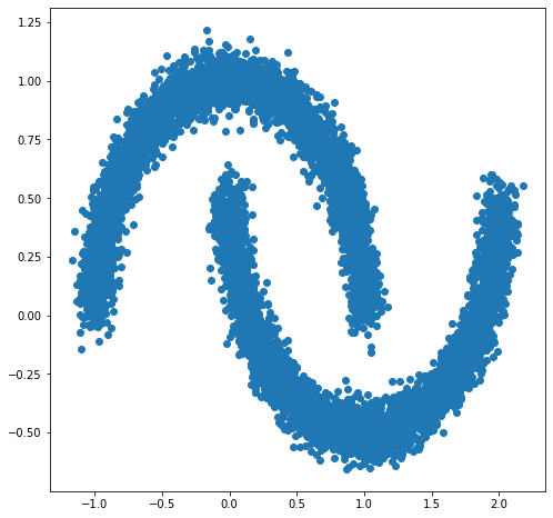
이 데모에서 우리는에 의해 정의 된 유통 위에 가우시안 분포 워프하는 FFJORD의 bijector을 훈련 할 것이다 moons 데이터 집합을. 이 작업은 3단계로 수행됩니다.
- 기본 분포를 정의
- FFJORD 바이젝터 정의
- 데이터 세트의 정확한 로그 가능성 최소화
먼저 데이터를 로드합니다.
데이터세트
DATASET_SIZE = 1024 * 8
BATCH_SIZE = 256
SAMPLE_SIZE = DATASET_SIZE

moons = skd.make_moons(n_samples=DATASET_SIZE, noise=.06)[0]

moons_ds = tf.data.Dataset.from_tensor_slices(moons.astype(np.float32))
moons_ds = moons_ds.prefetch(tf.data.experimental.AUTOTUNE)
moons_ds = moons_ds.cache()
moons_ds = moons_ds.shuffle(DATASET_SIZE)
moons_ds = moons_ds.batch(BATCH_SIZE)

plt.figure(figsize=[8, 8])
plt.scatter(moons[:, 0], moons[:, 1])
plt.show()
다음으로 기본 분포를 인스턴스화합니다.
base_loc = np.array([0.0, 0.0]).astype(np.float32)
base_sigma = np.array([0.8, 0.8]).astype(np.float32)
base_distribution = tfd.MultivariateNormalDiag(base_loc, base_sigma)
우리는 모델에 퍼셉트론 멀티 레이어를 사용 state_derivative_fn .
이 데이터 집합에 필요한 것은 아니지만, 그것을 만들기 위해 종종 benefitial입니다 state_derivative_fn 시간에 따라 다릅니다. 여기에서 우리는 연결하여이를 t 우리의 네트워크의 입력에.
class MLP_ODE(snt.Module):
  """Multi-layer NN ode_fn."""
  def __init__(self, num_hidden, num_layers, num_output, name='mlp_ode'):
    super(MLP_ODE, self).__init__(name=name)
    self._num_hidden = num_hidden
    self._num_output = num_output
    self._num_layers = num_layers
    self._modules = []
    for _ in range(self._num_layers - 1):
      self._modules.append(snt.Linear(self._num_hidden))
      self._modules.append(tf.math.tanh)
    self._modules.append(snt.Linear(self._num_output))
    self._model = snt.Sequential(self._modules)

  def __call__(self, t, inputs):
    inputs = tf.concat([tf.broadcast_to(t, inputs.shape), inputs], -1)
    return self._model(inputs)
모델 및 훈련 매개변수
LR = 1e-2
NUM_EPOCHS = 80
STACKED_FFJORDS = 4
NUM_HIDDEN = 8
NUM_LAYERS = 3
NUM_OUTPUT = 2
이제 FFJORD 바이젝터 스택을 구성합니다. 각 bijector이 제공된다 ode_solve_fn 및 trace_augmentation_fn 그것은 자신의 state_derivative_fn 서로 다른 변형의 순서를 나타냅니다 그래서, 모델.
건물 바이젝터
solver = tfp.math.ode.DormandPrince(atol=1e-5)
ode_solve_fn = solver.solve
trace_augmentation_fn = tfb.ffjord.trace_jacobian_exact

bijectors = []
for _ in range(STACKED_FFJORDS):
  mlp_model = MLP_ODE(NUM_HIDDEN, NUM_LAYERS, NUM_OUTPUT)
  next_ffjord = tfb.FFJORD(
      state_time_derivative_fn=mlp_model,ode_solve_fn=ode_solve_fn,
      trace_augmentation_fn=trace_augmentation_fn)
  bijectors.append(next_ffjord)

stacked_ffjord = tfb.Chain(bijectors[::-1])
이제 우리는 사용할 수 TransformedDistribution 뒤틀림의 결과 base_distribution 함께 stacked_ffjord bijector을.
transformed_distribution = tfd.TransformedDistribution(
    distribution=base_distribution, bijector=stacked_ffjord)
이제 훈련 절차를 정의합니다. 우리는 단순히 데이터의 음수 로그 가능성을 최소화합니다.
훈련
@tf.function
def train_step(optimizer, target_sample):
  with tf.GradientTape() as tape:
    loss = -tf.reduce_mean(transformed_distribution.log_prob(target_sample))
  variables = tape.watched_variables()
  gradients = tape.gradient(loss, variables)
  optimizer.apply(gradients, variables)
  return loss
시료
@tf.function
def get_samples():
  base_distribution_samples = base_distribution.sample(SAMPLE_SIZE)
  transformed_samples = transformed_distribution.sample(SAMPLE_SIZE)
  return base_distribution_samples, transformed_samples


@tf.function
def get_transformed_grid():
  transformed_grid = stacked_ffjord.forward(grid)
  return transformed_grid
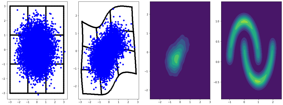
기본 및 변환된 분포에서 샘플을 플로팅합니다.
evaluation_samples = []
base_samples, transformed_samples = get_samples()
transformed_grid = get_transformed_grid()
evaluation_samples.append((base_samples, transformed_samples, transformed_grid))
WARNING:tensorflow:From /usr/local/lib/python3.6/dist-packages/tensorflow/python/ops/resource_variable_ops.py:1817: calling BaseResourceVariable.__init__ (from tensorflow.python.ops.resource_variable_ops) with constraint is deprecated and will be removed in a future version.
Instructions for updating:
If using Keras pass *_constraint arguments to layers.
panel_id = 0
panel_data = evaluation_samples[panel_id]
fig, axarray = plt.subplots(
  1, 4, figsize=(16, 6))
plot_panel(
    grid, panel_data[0], panel_data[2], panel_data[1], moons, axarray, False)
plt.tight_layout()
learning_rate = tf.Variable(LR, trainable=False)
optimizer = snt.optimizers.Adam(learning_rate)

for epoch in tqdm.trange(NUM_EPOCHS // 2):
  base_samples, transformed_samples = get_samples()
  transformed_grid = get_transformed_grid()
  evaluation_samples.append(
      (base_samples, transformed_samples, transformed_grid))
  for batch in moons_ds:
    _ = train_step(optimizer, batch)
0%|          | 0/40 [00:00<?, ?it/s]
WARNING:tensorflow:From /usr/local/lib/python3.6/dist-packages/tensorflow_probability/python/math/ode/base.py:350: calling while_loop_v2 (from tensorflow.python.ops.control_flow_ops) with back_prop=False is deprecated and will be removed in a future version.
Instructions for updating:
back_prop=False is deprecated. Consider using tf.stop_gradient instead.
Instead of:
results = tf.while_loop(c, b, vars, back_prop=False)
Use:
results = tf.nest.map_structure(tf.stop_gradient, tf.while_loop(c, b, vars))
100%|██████████| 40/40 [07:00<00:00, 10.52s/it]
panel_id = -1
panel_data = evaluation_samples[panel_id]
fig, axarray = plt.subplots(
  1, 4, figsize=(16, 6))
plot_panel(grid, panel_data[0], panel_data[2], panel_data[1], moons, axarray)
plt.tight_layout()
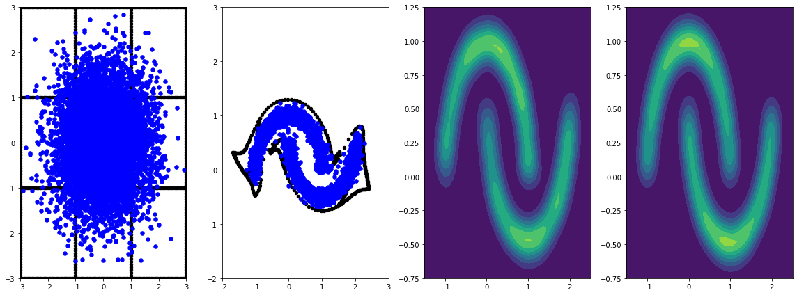
학습률로 더 오래 훈련하면 더 나은 결과를 얻을 수 있습니다.
이 예에서 변환되지 않은 FFJORD 바이젝터는 hutchinson의 확률적 추적 추정을 지원합니다. 특정 추정기를 통해 제공 될 수 trace_augmentation_fn . 마찬가지로 다른 통합이 커스텀 정의하여 사용할 수 ode_solve_fn .