팩토리얼 혼합물

TensorFlow.org에서 보기

Google Colab에서 실행

GitHub에서 소스 보기

노트북 다운로드

이 노트북에서 우리는 사용하는 방법을 보여 TensorFlow 확률 :로 정의 가우시안 분포의 계승 혼합물로부터 샘플 (TFP)을\(p(x_1, ..., x_n) = \prod_i p_i(x_i)\) 여기서 \(\begin{align*} p_i &\equiv \frac{1}{K}\sum_{k=1}^K \pi_{ik}\,\text{Normal}\left(\text{loc}=\mu_{ik},\, \text{scale}=\sigma_{ik}\right)\\1&=\sum_{k=1}^K\pi_{ik}, \forall i.\hphantom{MMMMMMMMMMM}\end{align*}\)

각 변수 \(x_i\) 가우시안 혼합하고 온통 조인트 분포로서 모델링된다 \(n\) 변수은 이러한 농도의 곱이다.

데이터 집합을 감안할 때 \(x^{(1)}, ..., x^{(T)}\), 우리는 각 dataponit 모델 \(x^{(j)}\) 가우시안의 계승 혼합물을 :

\[p(x^{(j)}) = \prod_i p_i (x_i^{(j)})\]

요인 혼합은 적은 수의 모수와 많은 수의 모드를 사용하여 분포를 생성하는 간단한 방법입니다.

import tensorflow as tf
import numpy as np
import tensorflow_probability as tfp
import matplotlib.pyplot as plt
import seaborn as sns
tfd = tfp.distributions

# Use try/except so we can easily re-execute the whole notebook.
try:
  tf.enable_eager_execution()
except:
  pass

TFP를 사용하여 가우스의 계승 혼합 만들기

num_vars = 2        # Number of variables (`n` in formula).
var_dim = 1         # Dimensionality of each variable `x[i]`.
num_components = 3  # Number of components for each mixture (`K` in formula).
sigma = 5e-2        # Fixed standard deviation of each component.

# Choose some random (component) modes.
component_mean = tfd.Uniform().sample([num_vars, num_components, var_dim])

factorial_mog = tfd.Independent(
   tfd.MixtureSameFamily(
       # Assume uniform weight on each component.
       mixture_distribution=tfd.Categorical(
           logits=tf.zeros([num_vars, num_components])),
       components_distribution=tfd.MultivariateNormalDiag(
           loc=component_mean, scale_diag=[sigma])),
   reinterpreted_batch_ndims=1)

우리의 사용에 주목 tfd.Independent . 이러한 "메타 분포"는 적용 reduce_sum 에 log_prob 가장 오른쪽 위에 계산 reinterpreted_batch_ndims 배치 크기. 우리가 계산 될 때 우리의 경우, 변수 아웃이 금액은 배치 차원을 떠나 차원 log_prob . 이것은 샘플링에 영향을 미치지 않습니다.

밀도 플로팅

점 그리드에서 밀도를 계산하고 모드의 위치를 빨간색 별과 함께 표시합니다. 요인 혼합의 각 모드는 기본 개별 변수 가우스 혼합의 모드 쌍에 해당합니다. 우리는 아래의 그래프에서 9 개 모드를 볼 수 있지만 우리는 6 개 매개 변수 필요 (의 모드의 위치 지정 3 \(x_1\), 그리고 3의 모드의 위치 지정 \(x_2\)). 대조적으로, 2 차원 공간에서의 가우시안 분포의 혼합물 \((x_1, x_2)\) 9 개 개의 모드를 지정하는 2 * 9 = 18 파라미터들을 요구한다.

plt.figure(figsize=(6,5))

# Compute density.
nx = 250 # Number of bins per dimension.
x = np.linspace(-3 * sigma, 1 + 3 * sigma, nx).astype('float32')
vals = tf.reshape(tf.stack(np.meshgrid(x, x), axis=2), (-1, num_vars, var_dim))
probs = factorial_mog.prob(vals).numpy().reshape(nx, nx)

# Display as image.
from matplotlib.colors import ListedColormap
cmap = ListedColormap(sns.color_palette("Blues", 256))
p = plt.pcolor(x, x, probs, cmap=cmap)
ax = plt.axis('tight');

# Plot locations of means.
means_np = component_mean.numpy().squeeze()
for mu_x in means_np[0]:
  for mu_y in means_np[1]:
    plt.scatter(mu_x, mu_y, s=150, marker='*', c='r', edgecolor='none');
plt.axis(ax);

plt.xlabel('$x_1$')
plt.ylabel('$x_2$')
plt.title('Density of factorial mixture of Gaussians');

png

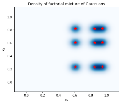
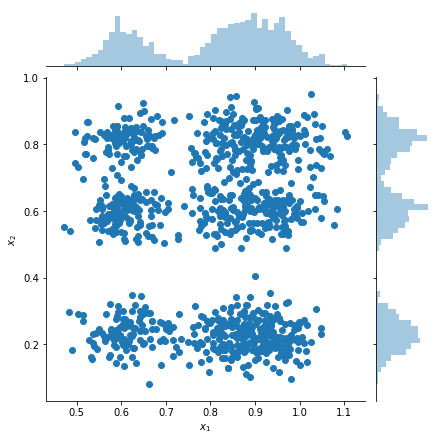
도표 표본 및 한계 밀도 추정치

samples = factorial_mog.sample(1000).numpy()

g = sns.jointplot(
    x=samples[:, 0, 0],
    y=samples[:, 1, 0],
    kind="scatter",
    marginal_kws=dict(bins=50))
g.set_axis_labels("$x_1$", "$x_2$");

png