
| | |  צפה במקור ב-GitHub צפה במקור ב-GitHub | |
import numpy as np
import matplotlib.pyplot as plt
import tensorflow.compat.v2 as tf
tf.enable_v2_behavior()

import tensorflow_probability as tfp
tfd = tfp.distributions
tfb = tfp.bijectors
A [קופולה"] (https://en.wikipedia.org/wiki/Copula_ (% probability_theory 29) היא גישה קלאסית ללכידת התלות בין משתנים אקראיים. נוסף רשמית, אוגד הוא ההתפלגות הרב \(C(U_1, U_2, ...., U_n)\) כך לשולי נותן \(U_i \sim \text{Uniform}(0, 1)\).
קופולים מעניינים מכיוון שאנו יכולים להשתמש בהם כדי ליצור התפלגויות רב-משתניות עם שוליים שרירותיים. זה המתכון:
- באמצעות אינטגרל הסתברות Transform תורות קרוונים רציפים שרירותי \(X\) לתוך מדים אחד \(F_X(X)\), שבו \(F_X\) הוא CDF של \(X\).
- בהתחשב אוגד (תניח שני משתנים) \(C(U, V)\), יש לנו כי \(U\) ו \(V\) יש הפצות שוליות אחידות.
- עכשיו נתון RV שלנו זה עניין \(X, Y\), ליצור הפצה חדש \(C'(X, Y) = C(F_X(X), F_Y(Y))\). השוליים עבור \(X\) ו \(Y\) הם אלה שאנחנו הרצוי.
השוליים הם חד משתנים ולכן עשויים להיות קלים יותר למדידה ו/או למודל. קופולה מאפשרת להתחיל משוליים אך גם להשיג מתאם שרירותי בין מימדים.
גאוס קופולה
כדי להמחיש כיצד בנויים קופולים, שקול את המקרה של לכידת תלות על פי מתאמים גאוסיים מרובי משתנים. גאוס קופולה" הוא אחד שנתן \(C(u_1, u_2, ...u_n) = \Phi_\Sigma(\Phi^{-1}(u_1), \Phi^{-1}(u_2), ... \Phi^{-1}(u_n))\) שבו \(\Phi_\Sigma\) מייצג את CDF של MultivariateNormal, עם השונות המשותפת \(\Sigma\) ולהתכוון 0, ו \(\Phi^{-1}\) הוא CDF ההופכי עבור הנורמלית הסטנדרטית.
החלת CDF הפוך של הנורמלי מעוותת את הממדים האחידים להתפלגות נורמלית. יישום ה-CDF של הנורמלי הרב-משתני מוחץ את ההתפלגות כך שתהיה אחידה בשוליים ועם מתאמים גאוסיים.
לכן, מה שאנחנו מקבלים זה כי גאוס קופולה" היא הפצה מעל קוביית יחידת \([0, 1]^n\) עם אנשי שולים אחידים.
מוגדר ככזה, את אוגד גאוס יכול להיות מיושם עם tfd.TransformedDistribution והולם Bijector . כלומר, אנו מבצעים שינוי MultivariateNormal, באמצעות שימוש ההתפלגות הנורמלית של ההופכי CDF, מיושם על ידי tfb.NormalCDF bijector.
להלן נבקש ליישם אוגד גאוס עם הנחת פישוט אחת: כי השונה המשותף הוא להם פרמטרים בפקטור Cholesky (ומכאן שונה המשותפת עבור MultivariateNormalTriL ). (אפשר להשתמש אחרים tf.linalg.LinearOperators לקודד נחות מטריקס חינם שונות.).
class GaussianCopulaTriL(tfd.TransformedDistribution):
"""Takes a location, and lower triangular matrix for the Cholesky factor."""
def __init__(self, loc, scale_tril):
super(GaussianCopulaTriL, self).__init__(
distribution=tfd.MultivariateNormalTriL(
loc=loc,
scale_tril=scale_tril),
bijector=tfb.NormalCDF(),
validate_args=False,
name="GaussianCopulaTriLUniform")
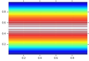
# Plot an example of this.
unit_interval = np.linspace(0.01, 0.99, num=200, dtype=np.float32)
x_grid, y_grid = np.meshgrid(unit_interval, unit_interval)
coordinates = np.concatenate(
[x_grid[..., np.newaxis],
y_grid[..., np.newaxis]], axis=-1)
pdf = GaussianCopulaTriL(
loc=[0., 0.],
scale_tril=[[1., 0.8], [0., 0.6]],
).prob(coordinates)
# Plot its density.
plt.contour(x_grid, y_grid, pdf, 100, cmap=plt.cm.jet);
עם זאת, הכוח ממודל כזה הוא שימוש ב-Probability Integral Transform, להשתמש ב-copula על RVs שרירותיים. בדרך זו, נוכל לציין שוליים שרירותיים, ולהשתמש ב-Cupula כדי לתפור אותם יחד.
נתחיל עם דגם:
\[\begin{align*} X &\sim \text{Kumaraswamy}(a, b) \\ Y &\sim \text{Gumbel}(\mu, \beta) \end{align*}\]
ולהשתמש קופולה" לקבל RV שני משתנים \(Z\), אשר יש השוליים Kumaraswamy ו Gumbel .
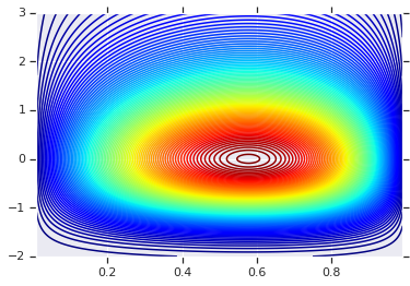
נתחיל בשרטוט התפלגות המוצר שנוצרה על ידי שני רכבי הפנאי הללו. זה רק כדי לשמש נקודת השוואה לזמן בו אנו מיישמים את ה-Copula.
a = 2.0
b = 2.0
gloc = 0.
gscale = 1.

x = tfd.Kumaraswamy(a, b)
y = tfd.Gumbel(loc=gloc, scale=gscale)

# Plot the distributions, assuming independence
x_axis_interval = np.linspace(0.01, 0.99, num=200, dtype=np.float32)
y_axis_interval = np.linspace(-2., 3., num=200, dtype=np.float32)
x_grid, y_grid = np.meshgrid(x_axis_interval, y_axis_interval)

pdf = x.prob(x_grid) * y.prob(y_grid)

# Plot its density

plt.contour(x_grid, y_grid, pdf, 100, cmap=plt.cm.jet);
חלוקה משותפת עם שוליים שונים
כעת אנו משתמשים בקופולה גאוסית כדי לחבר את ההפצות יחד, ולתכנן זאת. שוב הכלי של הבחירה שלנו היא TransformedDistribution יישום המתאים Bijector להשיג את השוליים שנבחר.
באופן ספציפי, אנו משתמשים Blockwise bijector אשר חל bijectors שונים בחלקים שונים של וקטור (שעדיין טרנספורמציה bijective).
עכשיו אנחנו יכולים להגדיר את הקופולה שאנחנו רוצים. בהינתן רשימה של שולי יעד (מקודדים כ-bijectors), נוכל בקלות לבנות התפלגות חדשה המשתמשת בקופולה ובעלת השוליים שצוינו.
class WarpedGaussianCopula(tfd.TransformedDistribution):
  """Application of a Gaussian Copula on a list of target marginals.

  This implements an application of a Gaussian Copula. Given [x_0, ... x_n]
  which are distributed marginally (with CDF) [F_0, ... F_n],
  `GaussianCopula` represents an application of the Copula, such that the
  resulting multivariate distribution has the above specified marginals.

  The marginals are specified by `marginal_bijectors`: These are
  bijectors whose `inverse` encodes the CDF and `forward` the inverse CDF.

  block_sizes is a 1-D Tensor to determine splits for `marginal_bijectors`
  length should be same as length of `marginal_bijectors`.
  See tfb.Blockwise for details
  """
  def __init__(self, loc, scale_tril, marginal_bijectors, block_sizes=None):
    super(WarpedGaussianCopula, self).__init__(
        distribution=GaussianCopulaTriL(loc=loc, scale_tril=scale_tril),
        bijector=tfb.Blockwise(bijectors=marginal_bijectors,
                               block_sizes=block_sizes),
        validate_args=False,
        name="GaussianCopula")
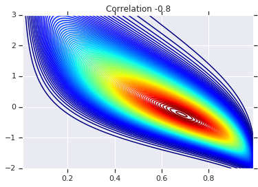
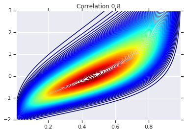
לבסוף, בואו נשתמש בעצם בקופולה גאוסית הזו. נשתמש Cholesky של \(\begin{bmatrix}1 & 0\\\rho & \sqrt{(1-\rho^2)}\end{bmatrix}\), אשר מתאים משונויות 1, ו קורלציה \(\rho\) עבור נורמלי המרובה משתנה.
נסתכל על כמה מקרים:
# Create our coordinates:
coordinates = np.concatenate(
[x_grid[..., np.newaxis], y_grid[..., np.newaxis]], -1)
def create_gaussian_copula(correlation):
# Use Gaussian Copula to add dependence.
return WarpedGaussianCopula(
loc=[0., 0.],
scale_tril=[[1., 0.], [correlation, tf.sqrt(1. - correlation ** 2)]],
# These encode the marginals we want. In this case we want X_0 has
# Kumaraswamy marginal, and X_1 has Gumbel marginal.
marginal_bijectors=[
tfb.Invert(tfb.KumaraswamyCDF(a, b)),
tfb.Invert(tfb.GumbelCDF(loc=0., scale=1.))])
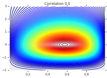
# Note that the zero case will correspond to independent marginals!
correlations = [0., -0.8, 0.8]
copulas = []
probs = []
for correlation in correlations:
copula = create_gaussian_copula(correlation)
copulas.append(copula)
probs.append(copula.prob(coordinates))
# Plot it's density
for correlation, copula_prob in zip(correlations, probs):
plt.figure()
plt.contour(x_grid, y_grid, copula_prob, 100, cmap=plt.cm.jet)
plt.title('Correlation {}'.format(correlation))
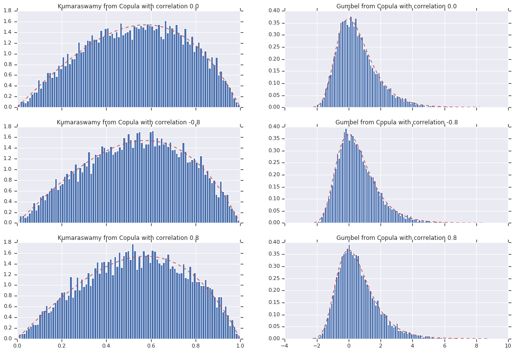
לבסוף, בואו נוודא שאנחנו באמת מקבלים את השוליים שאנחנו רוצים.
def kumaraswamy_pdf(x):
    return tfd.Kumaraswamy(a, b).prob(np.float32(x))

def gumbel_pdf(x):
    return tfd.Gumbel(gloc, gscale).prob(np.float32(x))


copula_samples = []
for copula in copulas:
  copula_samples.append(copula.sample(10000))

plot_rows = len(correlations)
plot_cols = 2  # for 2  densities [kumarswamy, gumbel]
fig, axes = plt.subplots(plot_rows, plot_cols, sharex='col', figsize=(18,12))

# Let's marginalize out on each, and plot the samples.

for i, (correlation, copula_sample) in enumerate(zip(correlations, copula_samples)):
  k = copula_sample[..., 0].numpy()
  g = copula_sample[..., 1].numpy()


  _, bins, _ = axes[i, 0].hist(k, bins=100, density=True)
  axes[i, 0].plot(bins, kumaraswamy_pdf(bins), 'r--')
  axes[i, 0].set_title('Kumaraswamy from Copula with correlation {}'.format(correlation))

  _, bins, _ = axes[i, 1].hist(g, bins=100, density=True)
  axes[i, 1].plot(bins, gumbel_pdf(bins), 'r--')
  axes[i, 1].set_title('Gumbel from Copula with correlation {}'.format(correlation))
סיכום
והנה אנחנו הולכים! הדגמנו כי נוכל לבנות גאוס Copulas באמצעות Bijector API.
באופן כללי יותר, כתיבת bijectors באמצעות Bijector API ולהלחין אותם עם ההפצה, יכול ליצור משפחות עשירות של הפצות עבור מודלים גמישים.