
| | |  GitHub에서 소스 보기 GitHub에서 소스 보기 | |
import numpy as np
import matplotlib.pyplot as plt
import tensorflow.compat.v2 as tf
tf.enable_v2_behavior()

import tensorflow_probability as tfp
tfd = tfp.distributions
tfb = tfp.bijectors
A [접합부 (https://en.wikipedia.org/wiki/Copula_ (probability_theory 29 %) 무작위 변수들과의 의존성을 포착 고전 접근법이다. 공식으로하는 접합부는 다변량 분포이다 \(C(U_1, U_2, ...., U_n)\) 주 변화되도록 제공 \(U_i \sim \text{Uniform}(0, 1)\).
Copulas는 임의의 한계가 있는 다변량 분포를 생성하는 데 사용할 수 있기 때문에 흥미롭습니다. 레시피는 다음과 같습니다.
- 은 Using 확률 적분 변환하는 회전을 임의의 연속 RV \(X\) 균일 하나로 \(F_X(X)\), \(F_X\) 의 CDF이다 \(X\).
- 접합부 (말 이변 량)을 감안할 때 \(C(U, V)\), 우리는이 \(U\) 및 \(V\) 균일 한계 분포를 가지고있다.
- 이제 우리의 RV이자의의 주어진 \(X, Y\)새 메일 작성, \(C'(X, Y) = C(F_X(X), F_Y(Y))\). 대한 marginals \(X\) 및 \(Y\) 우리가 원하는 것들입니다.
한계는 일변량이므로 측정 및/또는 모델링이 더 쉬울 수 있습니다. 코풀라를 사용하면 한계에서 시작하면서도 차원 간에 임의의 상관 관계를 달성할 수 있습니다.
가우스 코풀라
코풀러가 구성되는 방식을 설명하기 위해 다변량 가우스 상관 관계에 따라 종속성을 캡처하는 경우를 고려하십시오. 가우시안 접합부는 주어진 하나 \(C(u_1, u_2, ...u_n) = \Phi_\Sigma(\Phi^{-1}(u_1), \Phi^{-1}(u_2), ... \Phi^{-1}(u_n))\) \(\Phi_\Sigma\) 공분산 더불어 MultivariateNormal의 CDF를 나타낸다 \(\Sigma\) 및 평균 0 및 \(\Phi^{-1}\) 표준 정규 대한 역 CDF이다.
법선의 역 CDF를 적용하면 균일한 차원이 정규 분포를 따르도록 왜곡됩니다. 그런 다음 다변량 법선의 CDF를 적용하면 분포가 약간 균일하고 가우스 상관 관계가 있도록 압축됩니다.
따라서, 우리가 얻을 것은 가우스 접합부가 단위 하이퍼 큐브의 이상 분포이다 \([0, 1]^n\) 균일 marginals와.
같은 정의, 가우스 접합부가 구현 될 수 tfd.TransformedDistribution 적절한 Bijector . 즉 우리가 구현 한 정규 분포의 CDF 역의 사용을 통해하는 MultivariateNormal 변환되어있다 tfb.NormalCDF bijector.
아래, 우리는 하나의 단순화 가정하에 가우시안 접합부를 구현 : 공분산은 (따라서에 대한 공분산 촐레 요인에 의해 매개 변수화된다 MultivariateNormalTriL ). (하나는 다른 사용할 수 tf.linalg.LinearOperators 다른 매트릭스가없는 가정을 인코딩합니다.).
class GaussianCopulaTriL(tfd.TransformedDistribution):
"""Takes a location, and lower triangular matrix for the Cholesky factor."""
def __init__(self, loc, scale_tril):
super(GaussianCopulaTriL, self).__init__(
distribution=tfd.MultivariateNormalTriL(
loc=loc,
scale_tril=scale_tril),
bijector=tfb.NormalCDF(),
validate_args=False,
name="GaussianCopulaTriLUniform")
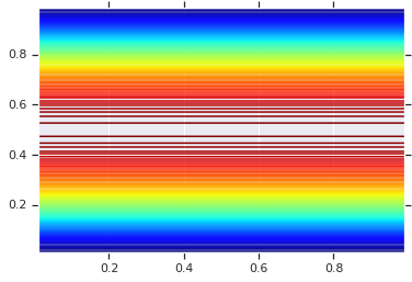
# Plot an example of this.
unit_interval = np.linspace(0.01, 0.99, num=200, dtype=np.float32)
x_grid, y_grid = np.meshgrid(unit_interval, unit_interval)
coordinates = np.concatenate(
[x_grid[..., np.newaxis],
y_grid[..., np.newaxis]], axis=-1)
pdf = GaussianCopulaTriL(
loc=[0., 0.],
scale_tril=[[1., 0.8], [0., 0.6]],
).prob(coordinates)
# Plot its density.
plt.contour(x_grid, y_grid, pdf, 100, cmap=plt.cm.jet);
그러나 이러한 모델의 힘은 확률 적분 변환을 사용하여 임의의 RV에 코풀라를 사용하는 것입니다. 이러한 방식으로 임의의 한계를 지정하고 코퓰러를 사용하여 함께 연결할 수 있습니다.
우리는 모델로 시작합니다.
\[\begin{align*} X &\sim \text{Kumaraswamy}(a, b) \\ Y &\sim \text{Gumbel}(\mu, \beta) \end{align*}\]
그리고 이변의 RV를 얻기 위해 접합부를 사용 \(Z\)marginals 가지고, Kumaraswamy 와 Gumbel와를 .
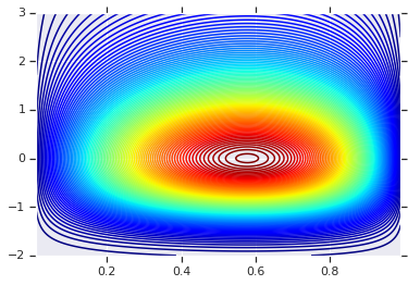
이 두 RV에 의해 생성된 제품 분포를 플로팅하는 것으로 시작하겠습니다. 이것은 Copula를 적용할 때 비교 지점으로 사용하기 위한 것입니다.
a = 2.0
b = 2.0
gloc = 0.
gscale = 1.

x = tfd.Kumaraswamy(a, b)
y = tfd.Gumbel(loc=gloc, scale=gscale)

# Plot the distributions, assuming independence
x_axis_interval = np.linspace(0.01, 0.99, num=200, dtype=np.float32)
y_axis_interval = np.linspace(-2., 3., num=200, dtype=np.float32)
x_grid, y_grid = np.meshgrid(x_axis_interval, y_axis_interval)

pdf = x.prob(x_grid) * y.prob(y_grid)

# Plot its density

plt.contour(x_grid, y_grid, pdf, 100, cmap=plt.cm.jet);
다른 한계를 가진 공동 분배
이제 가우스 코풀러를 사용하여 분포를 함께 연결하고 플롯합니다. 다시 선택의 우리의 도구입니다 TransformedDistribution 적절한 적용 Bijector 선택한 marginals을 얻었다.
구체적으로 우리가 사용하는 Blockwise (여전히 전단 사 변환이다) 벡터의 서로 다른 부분에서 서로 다른 적용 bijectors bijector한다.
이제 원하는 Copula를 정의할 수 있습니다. 목표 한계(바이젝터로 인코딩됨) 목록이 주어지면 코풀라를 사용하고 지정된 한계를 갖는 새 분포를 쉽게 구성할 수 있습니다.
class WarpedGaussianCopula(tfd.TransformedDistribution):
  """Application of a Gaussian Copula on a list of target marginals.

  This implements an application of a Gaussian Copula. Given [x_0, ... x_n]
  which are distributed marginally (with CDF) [F_0, ... F_n],
  `GaussianCopula` represents an application of the Copula, such that the
  resulting multivariate distribution has the above specified marginals.

  The marginals are specified by `marginal_bijectors`: These are
  bijectors whose `inverse` encodes the CDF and `forward` the inverse CDF.

  block_sizes is a 1-D Tensor to determine splits for `marginal_bijectors`
  length should be same as length of `marginal_bijectors`.
  See tfb.Blockwise for details
  """
  def __init__(self, loc, scale_tril, marginal_bijectors, block_sizes=None):
    super(WarpedGaussianCopula, self).__init__(
        distribution=GaussianCopulaTriL(loc=loc, scale_tril=scale_tril),
        bijector=tfb.Blockwise(bijectors=marginal_bijectors,
                               block_sizes=block_sizes),
        validate_args=False,
        name="GaussianCopula")
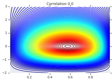
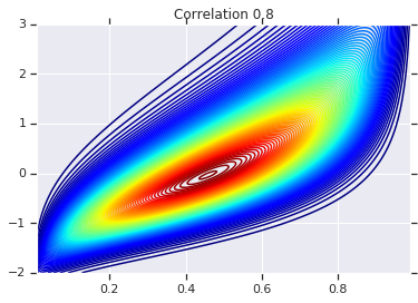
마지막으로 이 가우스 코풀라를 실제로 사용해 봅시다. 우리는의 콜레 사용합니다 \(\begin{bmatrix}1 & 0\\\rho & \sqrt{(1-\rho^2)}\end{bmatrix}\)1 편차를에 해당됩니다,와 상관 \(\rho\) 다변량 정상을 위해.
몇 가지 경우를 살펴보겠습니다.
# Create our coordinates:
coordinates = np.concatenate(
[x_grid[..., np.newaxis], y_grid[..., np.newaxis]], -1)
def create_gaussian_copula(correlation):
# Use Gaussian Copula to add dependence.
return WarpedGaussianCopula(
loc=[0., 0.],
scale_tril=[[1., 0.], [correlation, tf.sqrt(1. - correlation ** 2)]],
# These encode the marginals we want. In this case we want X_0 has
# Kumaraswamy marginal, and X_1 has Gumbel marginal.
marginal_bijectors=[
tfb.Invert(tfb.KumaraswamyCDF(a, b)),
tfb.Invert(tfb.GumbelCDF(loc=0., scale=1.))])
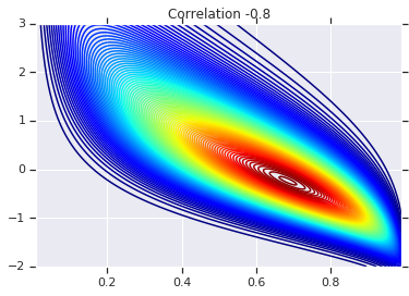
# Note that the zero case will correspond to independent marginals!
correlations = [0., -0.8, 0.8]
copulas = []
probs = []
for correlation in correlations:
copula = create_gaussian_copula(correlation)
copulas.append(copula)
probs.append(copula.prob(coordinates))
# Plot it's density
for correlation, copula_prob in zip(correlations, probs):
plt.figure()
plt.contour(x_grid, y_grid, copula_prob, 100, cmap=plt.cm.jet)
plt.title('Correlation {}'.format(correlation))
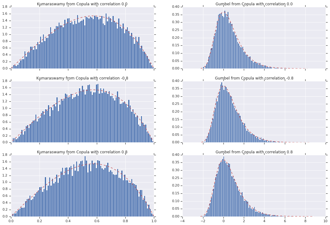
마지막으로 원하는 한계값을 실제로 얻었는지 확인하겠습니다.
def kumaraswamy_pdf(x):
    return tfd.Kumaraswamy(a, b).prob(np.float32(x))

def gumbel_pdf(x):
    return tfd.Gumbel(gloc, gscale).prob(np.float32(x))


copula_samples = []
for copula in copulas:
  copula_samples.append(copula.sample(10000))

plot_rows = len(correlations)
plot_cols = 2  # for 2  densities [kumarswamy, gumbel]
fig, axes = plt.subplots(plot_rows, plot_cols, sharex='col', figsize=(18,12))

# Let's marginalize out on each, and plot the samples.

for i, (correlation, copula_sample) in enumerate(zip(correlations, copula_samples)):
  k = copula_sample[..., 0].numpy()
  g = copula_sample[..., 1].numpy()


  _, bins, _ = axes[i, 0].hist(k, bins=100, density=True)
  axes[i, 0].plot(bins, kumaraswamy_pdf(bins), 'r--')
  axes[i, 0].set_title('Kumaraswamy from Copula with correlation {}'.format(correlation))

  _, bins, _ = axes[i, 1].hist(g, bins=100, density=True)
  axes[i, 1].plot(bins, gumbel_pdf(bins), 'r--')
  axes[i, 1].set_title('Gumbel from Copula with correlation {}'.format(correlation))
결론
그리고 우리는 간다! 우리는 우리가 사용하는 가우스 Copulas를 구성 할 수 있음을 입증 한 Bijector API를.
더 일반적으로, bijectors 사용하여 작성 Bijector 유연한 모델링을위한 배포판의 부유 한 가족을 만들 수 있습니다, API 및 유통로를 구성합니다.