
| | |  GitHub에서 소스 보기 GitHub에서 소스 보기 | |
잠재 변수 모델은 고차원 데이터의 숨겨진 구조를 캡처하려고 시도합니다. 예로는 PCA(주성분 분석) 및 요인 분석이 있습니다. 가우스 프로세스는 로컬 상관 구조와 불확실성을 유연하게 포착할 수 있는 "비모수적" 모델입니다. 가우시안 과정 잠재 변수 모델 ( 로렌스, 2004 ) 이러한 개념을 결합한다.
배경: 가우스 프로세스
가우스 과정은 임의의 유한 부분 집합에 대한 주변 분포가 다변량 정규 분포가 되도록 하는 임의의 변수 모음입니다. 회귀 분석의 맥락에서 개업을 자세히 살펴 들어, 체크 아웃 TensorFlow 확률의 가우시안 프로세스 회귀를 .
우리는 GP를 포함하는 컬렉션의 확률 변수의 각 레이블을 소위 인덱스 세트를 사용합니다. 유한 인덱스 세트의 경우 다변량 법선을 얻습니다. 우리는 무한 컬렉션을 고려할 때 GP 년대는하지만, 가장 흥미로운 있습니다. 같은 인덱스 세트의 경우 \(\mathbb{R}^D\)우리의 모든 단계에 대한 임의의 변수가, \(D\)차원 공간의 GP는 랜덤 기능을 통해 유통으로 간주 할 수 있습니다. 등의 GP에서 하나의 무승부는, 그것이 실현 될 수 있다면, 모든 점에 (공동 일반적으로 분산) 값을 할당합니다 \(\mathbb{R}^D\). 이 colab에서, 우리는 몇 가지에 걸쳐 GP의에 초점을 맞출 것이다\(\mathbb{R}^D\).
정규 분포는 1차 및 2차 통계에 의해 완전히 결정됩니다. 실제로 정규 분포를 정의하는 한 가지 방법은 고차 누적량이 모두 0인 방법입니다. 이 역시, GP의의 경우입니다 : 우리가 완전히 평균과 공분산 *을 설명하여 GP를 지정합니다. 유한 차원 다변량 법선의 경우 평균은 벡터이고 공분산은 정방형 양의 정부호 대칭 행렬입니다. 무한 차원 GP, 이러한 구조는 평균 함수로 일반화 \(m : \mathbb{R}^D \to \mathbb{R}\)인덱스 세트의 각 점에서 정의 및 공분산 "커널"기능,\(k : \mathbb{R}^D \times \mathbb{R}^D \to \mathbb{R}\). 커널 함수가 될 필요 포지티브 명확한 본질적 것을 말한다되는 점의 유한 세트에 한정 그것은 postiive-일정한 매트릭스를 산출.
GP 구조의 대부분은 공분산 커널 함수에서 파생됩니다. 이 함수는 샘플 함수의 값이 가까운(또는 가깝지 않은) 지점에서 어떻게 변하는지 설명합니다. 다른 공분산 함수는 다른 정도의 평활도를 촉진합니다. 하나 개의 일반적으로 사용되는 커널 함수는 "거듭 제곱 차"(일명 "가우시안"또는 "방사형 기저 함수" "지수 제곱")이다 \(k(x, x') = \sigma^2 e^{(x - x^2) / \lambda^2}\). 다른 예로는 데이비드 Duvenaud의에 설명되어 커널 요리 책 페이지 정식 텍스트뿐만 아니라, 기계 학습을위한 가우스 프로세스 .
* 무한 인덱스 세트를 사용하면 일관성 조건도 필요합니다. GP의 정의는 유한한 한계의 관점에서 이루어지기 때문에 우리는 이러한 한계가 한계를 취하는 순서와 상관없이 일관되어야 한다고 요구해야 합니다. 이것은 이 튜토리얼의 범위를 벗어나는 확률적 과정 이론의 다소 고급 주제입니다. 결국 일이 잘 풀린다고 말하는 것으로 충분합니다!
GP 적용: 회귀 및 잠재 변수 모델
우리가 GPS를 사용할 수있는 한 가지 방법은 회귀를위한 것입니다 입력의 형태로 관찰 된 데이터의 무리 주어진 \(\{x_i\}_{i=1}^N\) (인덱스 세트의 요소)과 관찰\(\{y_i\}_{i=1}^N\), 우리는 이러한 새로운에서 사후 예측 분포를 형성하는 데 사용할 수있는 점의 세트는 \(\{x_j^*\}_{j=1}^M\). 배포판은 모든 가우스을하기 때문에,이 몇 가지 간단한 선형 대수로 요약된다 (그러나 참고 : 필요한 계산은 데이터 포인트의 수 런타임 입방이 데이터 포인트의 수 공간의 차를 필요 -이 주요 제한 요인으로는 GP의 사용과 현재의 많은 연구는 정확한 사후 추론에 대한 계산적으로 실행 가능한 대안에 중점을 둡니다. 우리는 더 자세히 GP의 회귀를 포함 총요소 생산성 colab에서 GP 회귀 .
GP를 사용할 수 있는 또 다른 방법은 잠재 변수 모델로 사용하는 것입니다. 고차원 관찰(예: 이미지) 모음이 주어지면 일부 저차원 잠재 구조를 포지셔닝할 수 있습니다. 잠재 구조에 따라 많은 수의 출력(이미지의 픽셀)이 서로 독립적이라고 가정합니다. 이 모델의 교육은 다음으로 구성됩니다.
- 모델 매개변수 최적화(커널 함수 매개변수 및 관찰 잡음 분산),
- 각 훈련 관찰(이미지)에 대해 인덱스 세트에서 해당 지점 위치를 찾습니다. 모든 최적화는 데이터의 한계 로그 가능성을 최대화하여 수행할 수 있습니다.
수입품
import numpy as np
import tensorflow.compat.v2 as tf
tf.enable_v2_behavior()
import tensorflow_probability as tfp
tfd = tfp.distributions
tfk = tfp.math.psd_kernels
%pylab inline
Populating the interactive namespace from numpy and matplotlib
MNIST 데이터 로드
# Load the MNIST data set and isolate a subset of it.
(x_train, y_train), (_, _) = tf.keras.datasets.mnist.load_data()
N = 1000
small_x_train = x_train[:N, ...].astype(np.float64) / 256.
small_y_train = y_train[:N]
Downloading data from https://storage.googleapis.com/tensorflow/tf-keras-datasets/mnist.npz
11493376/11490434 [==============================] - 0s 0us/step
11501568/11490434 [==============================] - 0s 0us/step
훈련 가능한 변수 준비
우리는 3개의 모델 매개변수와 잠재 입력을 공동으로 훈련할 것입니다.
# Create some trainable model parameters. We will constrain them to be strictly
# positive when constructing the kernel and the GP.
unconstrained_amplitude = tf.Variable(np.float64(1.), name='amplitude')
unconstrained_length_scale = tf.Variable(np.float64(1.), name='length_scale')
unconstrained_observation_noise = tf.Variable(np.float64(1.), name='observation_noise')
# We need to flatten the images and, somewhat unintuitively, transpose from
# shape [100, 784] to [784, 100]. This is because the 784 pixels will be
# treated as *independent* conditioned on the latent inputs, meaning we really
# have a batch of 784 GP's with 100 index_points.
observations_ = small_x_train.reshape(N, -1).transpose()

# Create a collection of N 2-dimensional index points that will represent our
# latent embeddings of the data. (Lawrence, 2004) prescribes initializing these
# with PCA, but a random initialization actually gives not-too-bad results, so
# we use this for simplicity. For a fun exercise, try doing the
# PCA-initialization yourself!
init_ = np.random.normal(size=(N, 2))
latent_index_points = tf.Variable(init_, name='latent_index_points')
모델 구성 및 학습 작업
# Create our kernel and GP distribution
EPS = np.finfo(np.float64).eps

def create_kernel():
  amplitude = tf.math.softplus(EPS + unconstrained_amplitude)
  length_scale = tf.math.softplus(EPS + unconstrained_length_scale)
  kernel = tfk.ExponentiatedQuadratic(amplitude, length_scale)
  return kernel

def loss_fn():
  observation_noise_variance = tf.math.softplus(
      EPS + unconstrained_observation_noise)
  gp = tfd.GaussianProcess(
      kernel=create_kernel(),
      index_points=latent_index_points,
      observation_noise_variance=observation_noise_variance)
  log_probs = gp.log_prob(observations_, name='log_prob')
  return -tf.reduce_mean(log_probs)

trainable_variables = [unconstrained_amplitude,
                       unconstrained_length_scale,
                       unconstrained_observation_noise,
                       latent_index_points]

optimizer = tf.optimizers.Adam(learning_rate=1.0)

@tf.function(autograph=False, jit_compile=True)
def train_model():
  with tf.GradientTape() as tape:
    loss_value = loss_fn()
  grads = tape.gradient(loss_value, trainable_variables)
  optimizer.apply_gradients(zip(grads, trainable_variables))
  return loss_value
결과 잠재 임베딩 훈련 및 플로팅
# Initialize variables and train!
num_iters = 100
log_interval = 20
lips = np.zeros((num_iters, N, 2), np.float64)
for i in range(num_iters):
  loss = train_model()
  lips[i] = latent_index_points.numpy()
  if i % log_interval == 0 or i + 1 == num_iters:
    print("Loss at step %d: %f" % (i, loss))
Loss at step 0: 1108.121688
Loss at step 20: -159.633761
Loss at step 40: -263.014394
Loss at step 60: -283.713056
Loss at step 80: -288.709413
Loss at step 99: -289.662253
플롯 결과
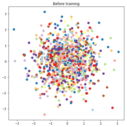
# Plot the latent locations before and after training
plt.figure(figsize=(7, 7))
plt.title("Before training")
plt.grid(False)
plt.scatter(x=init_[:, 0], y=init_[:, 1],
c=y_train[:N], cmap=plt.get_cmap('Paired'), s=50)
plt.show()
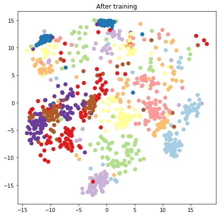
plt.figure(figsize=(7, 7))
plt.title("After training")
plt.grid(False)
plt.scatter(x=lips[-1, :, 0], y=lips[-1, :, 1],
c=y_train[:N], cmap=plt.get_cmap('Paired'), s=50)
plt.show()
예측 모델 및 샘플링 작업 구성
# We'll draw samples at evenly spaced points on a 10x10 grid in the latent
# input space.
sample_grid_points = 10
grid_ = np.linspace(-4, 4, sample_grid_points).astype(np.float64)
# Create a 10x10 grid of 2-vectors, for a total shape [10, 10, 2]
grid_ = np.stack(np.meshgrid(grid_, grid_), axis=-1)

# This part's a bit subtle! What we defined above was a batch of 784 (=28x28)
# independent GP distributions over the input space. Each one corresponds to a
# single pixel of an MNIST image. Now what we'd like to do is draw 100 (=10x10)
# *independent* samples, each one separately conditioned on all the observations
# as well as the learned latent input locations above.
#
# The GP regression model below will define a batch of 784 independent
# posteriors. We'd like to get 100 independent samples each at a different
# latent index point. We could loop over the points in the grid, but that might
# be a bit slow. Instead, we can vectorize the computation by tacking on *even
# more* batch dimensions to our GaussianProcessRegressionModel distribution.
# In the below grid_ shape, we have concatentaed
#   1. batch shape: [sample_grid_points, sample_grid_points, 1]
#   2. number of examples: [1]
#   3. number of latent input dimensions: [2]
# The `1` in the batch shape will broadcast with 784. The final result will be
# samples of shape [10, 10, 784, 1]. The `1` comes from the "number of examples"
# and we can just `np.squeeze` it off.
grid_ = grid_.reshape(sample_grid_points, sample_grid_points, 1, 1, 2)

# Create the GPRegressionModel instance which represents the posterior
# predictive at the grid of new points.
gprm = tfd.GaussianProcessRegressionModel(
    kernel=create_kernel(),
    # Shape [10, 10, 1, 1, 2]
    index_points=grid_,
    # Shape [1000, 2]. 1000 2 dimensional vectors.
    observation_index_points=latent_index_points,
    # Shape [784, 1000]. A batch of 784 1000-dimensional observations.
    observations=observations_)
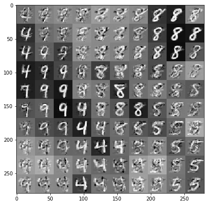
데이터 및 잠재 임베딩을 조건으로 하는 샘플 그리기
잠재 공간의 2차원 그리드에서 100개 지점에서 샘플링합니다.
samples = gprm.sample()

# Plot the grid of samples at new points. We do a bit of tweaking of the samples
# first, squeezing off extra 1-shapes and normalizing the values.
samples_ = np.squeeze(samples.numpy())
samples_ = ((samples_ -
             samples_.min(-1, keepdims=True)) /
            (samples_.max(-1, keepdims=True) -
             samples_.min(-1, keepdims=True)))
samples_ = samples_.reshape(sample_grid_points, sample_grid_points, 28, 28)
samples_ = samples_.transpose([0, 2, 1, 3])
samples_ = samples_.reshape(28 * sample_grid_points, 28 * sample_grid_points)
plt.figure(figsize=(7, 7))
ax = plt.subplot()
ax.grid(False)
ax.imshow(-samples_, interpolation='none', cmap='Greys')
plt.show()
결론
우리는 가우스 프로세스 잠재 변수 모델을 간략하게 살펴보고 TF 및 TF 확률 코드 몇 줄로 이를 구현하는 방법을 보여주었습니다.