
| | |  צפה במקור ב-GitHub צפה במקור ב-GitHub | |
בקולאב זה, אנו חוקרים רגרסיה של תהליך גאוס באמצעות TensorFlow ו- TensorFlow Probability. אנו מייצרים כמה תצפיות רועשות מכמה פונקציות ידועות ומתאים מודלים של GP לנתונים אלה. לאחר מכן אנו דוגמים מהרופא האחורי ומשרטטים את ערכי הפונקציות שנדגמו על פני רשתות בתחומים שלהם.
רקע כללי
בואו \(\mathcal{X}\) להיות כל קבוצה. תהליך גאוס (GP) הוא אוסף של משתנים אקראיים באינדקס \(\mathcal{X}\) כזה שאם\(\{X_1, \ldots, X_n\} \subset \mathcal{X}\) הוא כול תת-קבוצה סופית, הצפיפות השולית\(p(X_1 = x_1, \ldots, X_n = x_n)\) הוא גאוס מרובה משתנה. כל התפלגות גאוסית מוגדרת לחלוטין על ידי הרגע המרכזי הראשון והשני שלה (ממוצע ושונות), והרופאים אינם יוצאי דופן. אנחנו יכולים לציין GP לחלוטין מבחינת התפקוד הממוצע שלה \(\mu : \mathcal{X} \to \mathbb{R}\) ואת השונות המשותפת פונקציה\(k : \mathcal{X} \times \mathcal{X} \to \mathbb{R}\). רוב כוח ההבעה של רופאי משפחה מובלע בבחירה של פונקציית שיתוף פעולה. מסיבות שונות, את הפונקציה השונה המשותפת נקראת גם כפונקציה הקרנל. זה נדרש רק כדי להיות סימטרי וחיובי-ברור (ראה Ch. 4 של רסמוסן & Williams ). להלן אנו עושים שימוש בליבת קוvariance ExponentiatedQuadratic. צורתו היא
\[ k(x, x') := \sigma^2 \exp \left( \frac{\|x - x'\|^2}{\lambda^2} \right) \]
שם \(\sigma^2\) נקרא "משרעת" ו \(\lambda\) בקנה מידת האורך. ניתן לבחור את פרמטרי הליבה באמצעות הליך אופטימיזציה של סבירות מקסימלית.
מדגם מלא של GP כוללת פונקציה ממשית על המרחב כולו\(\mathcal{X}\) והוא בפועל מעשי לממש; לעתים קרובות בוחרים קבוצה של נקודות שבהן ניתן לצפות במדגם ומציירים ערכי פונקציה בנקודות אלו. זה מושג על ידי דגימה מגאוס רב משתנים מתאים (סופי ממדי).
שימו לב שלפי ההגדרה לעיל, כל התפלגות גאוסית סופי ממדי רב-משתנים היא גם תהליך גאוסי. בדרך כלל, כאשר אחד מתייחס GP, זה משתמע כי מערך המדד הוא כמה \(\mathbb{R}^n\)ואנחנו אכן נעשה הנחה זו כאן.
יישום נפוץ של תהליכי גאוס בלמידת מכונה הוא רגרסיית תהליכי גאוס. הרעיון הוא שאנחנו רוצים להעריך פונקציה ידוע נתון תצפיות רועש \(\{y_1, \ldots, y_N\}\) של הפונקציה בכל מספר סופי של נקודות \(\{x_1, \ldots x_N\}.\) אנו לדמיין תהליך יוֹצֵר
\[ \begin{align} f \sim \: & \textsf{GaussianProcess}\left( \text{mean_fn}=\mu(x), \text{covariance_fn}=k(x, x')\right) \\ y_i \sim \: & \textsf{Normal}\left( \text{loc}=f(x_i), \text{scale}=\sigma\right), i = 1, \ldots, N \end{align} \]
כפי שצוין לעיל, הפונקציה הדגימה בלתי אפשרית לחישוב, מכיוון שהיינו דורשים את ערכה במספר אינסופי של נקודות. במקום זאת, רואים מדגם סופי מגאוס רב משתנים.
\[ \begin{gather} \begin{bmatrix} f(x_1) \\ \vdots \\ f(x_N) \end{bmatrix} \sim \textsf{MultivariateNormal} \left( \: \text{loc}= \begin{bmatrix} \mu(x_1) \\ \vdots \\ \mu(x_N) \end{bmatrix} \:,\: \text{scale}= \begin{bmatrix} k(x_1, x_1) & \cdots & k(x_1, x_N) \\ \vdots & \ddots & \vdots \\ k(x_N, x_1) & \cdots & k(x_N, x_N) \\ \end{bmatrix}^{1/2} \: \right) \end{gather} \\ y_i \sim \textsf{Normal} \left( \text{loc}=f(x_i), \text{scale}=\sigma \right) \]
הערת המעריך \(\frac{1}{2}\) על המטריצה: זו מציינת פירוק שולסקי. חישוב ה-Cholesky הכרחי מכיוון שה-MVN הוא הפצה משפחתית בקנה מידה של מיקום. למרבה הצער פירוק שולסקי הוא יקר המחשוב, לקיחת \(O(N^3)\) זמן \(O(N^2)\) החלל. חלק ניכר מהספרות של רופאי המשפחה מתמקד בהתמודדות עם המעריך הקטן התמים לכאורה הזה.
מקובל לקחת את הפונקציה הממוצעת הקודמת להיות קבועה, לעתים קרובות אפס. כמו כן, כמה מוסכמות סימון הן נוחות. אחת קרובות כותב \(\mathbf{f}\) עבור הווקטור הסופי של ערכי פונקצית שנדגמו. מספר הסימונים המעניינים משמש עבור מטריצת נובע מהיישום של \(k\) לצמדי תשומות. בעקבות (Quiñonero-קנדלה, 2005) , נציין כי הרכיבים של המטריצה הם שונים משותפים של ערכי פונקציה בנקודה קלט מסוימים. לכן אנו יכולים לציין את המטריצה כמו \(K_{AB}\)שבו \(A\) ו \(B\) כמה אינדיקטורים של האוסף של ערכי פונקציה לאורך ממדי מטריקס נתון.
לדוגמה, נתונים נצפים נתון \((\mathbf{x}, \mathbf{y})\) עם ערכי פונקציה סמויה משתמעת \(\mathbf{f}\), נוכל לכתוב
\[ K_{\mathbf{f},\mathbf{f} } = \begin{bmatrix} k(x_1, x_1) & \cdots & k(x_1, x_N) \\ \vdots & \ddots & \vdots \\ k(x_N, x_1) & \cdots & k(x_N, x_N) \\ \end{bmatrix} \]
באופן דומה, אנו יכולים לערבב קבוצות של תשומות, כמו ב
\[ K_{\mathbf{f},*} = \begin{bmatrix} k(x_1, x^*_1) & \cdots & k(x_1, x^*_T) \\ \vdots & \ddots & \vdots \\ k(x_N, x^*_1) & \cdots & k(x_N, x^*_T) \\ \end{bmatrix} \]
איפה אנחנו, מסתבר שיש \(N\) תשומות ההכשרה, וכן \(T\) תשומות המבחן. התהליך הגנרטיבי לעיל עשוי להיכתב בצורה קומפקטית בשם
\[ \begin{align} \mathbf{f} \sim \: & \textsf{MultivariateNormal} \left( \text{loc}=\mathbf{0}, \text{scale}=K_{\mathbf{f},\mathbf{f} }^{1/2} \right) \\ y_i \sim \: & \textsf{Normal} \left( \text{loc}=f_i, \text{scale}=\sigma \right), i = 1, \ldots, N \end{align} \]
מבצע הדגימה בשורה הראשונה מניב קבוצה סופית של \(N\) ערכי פונקציה של גאוס מרובה משתנית - לא פונקציה כול כמו מעל GP סימון לצייר. השורה השנייה מתאר אוסף של \(N\) שואבת מן Gaussians משתנה אחד מרוכז על ערכי פונקציה שונים, עם רעש תצפית קבועה \(\sigma^2\).
עם המודל הגנרטיבי לעיל, נוכל להמשיך לשקול את בעיית ההסקה האחורית. זה מניב התפלגות אחורית על ערכי תפקוד בקבוצה חדשה של נקודות בדיקה, המותנה על הנתונים הרועשים שנצפו מהתהליך שלמעלה.
עם הכיתוב הנ"ל במקום, אנחנו יכולים לכתוב על חלוק חזוי האחורית בצורה מרוכזת על עתידו (רועשות) תצפיות מותנות המקביל תשומות ונתוני אימון כדלקמן (לפרטים נוספים, ראה §2.2 של רסמוסן & Williams ).
\[ \mathbf{y}^* \mid \mathbf{x}^*, \mathbf{x}, \mathbf{y} \sim \textsf{Normal} \left( \text{loc}=\mathbf{\mu}^*, \text{scale}=(\Sigma^*)^{1/2} \right), \]
איפה
\[ \mathbf{\mu}^* = K_{*,\mathbf{f} }\left(K_{\mathbf{f},\mathbf{f} } + \sigma^2 I \right)^{-1} \mathbf{y} \]
ו
\[ \Sigma^* = K_{*,*} - K_{*,\mathbf{f} } \left(K_{\mathbf{f},\mathbf{f} } + \sigma^2 I \right)^{-1} K_{\mathbf{f},*} \]
יבוא
import time

import numpy as np
import matplotlib.pyplot as plt
import tensorflow.compat.v2 as tf
import tensorflow_probability as tfp
tfb = tfp.bijectors
tfd = tfp.distributions
tfk = tfp.math.psd_kernels
tf.enable_v2_behavior()

from mpl_toolkits.mplot3d import Axes3D
%pylab inline
# Configure plot defaults
plt.rcParams['axes.facecolor'] = 'white'
plt.rcParams['grid.color'] = '#666666'
%config InlineBackend.figure_format = 'png'
Populating the interactive namespace from numpy and matplotlib
דוגמה: רגרסיה מדויקת של GP על נתונים סינוסואידיים רועשים
כאן אנו מייצרים נתוני אימון מסינוסואיד רועש, ואז דוגמים חבורה של עקומות מהחלק האחורי של מודל הרגרסיה של GP. אנו משתמשים אדם כדי לייעל את hyperparameters הקרנל (אנו למזער את סבירות היומן השלילית של הנתונים תחת המוקדם). אנו משרטטים את עקומת האימון, ואחריה את הפונקציה האמיתית והדגימות האחוריות.
def sinusoid(x):
  return np.sin(3 * np.pi * x[..., 0])

def generate_1d_data(num_training_points, observation_noise_variance):
  """Generate noisy sinusoidal observations at a random set of points.

  Returns:
     observation_index_points, observations
  """
  index_points_ = np.random.uniform(-1., 1., (num_training_points, 1))
  index_points_ = index_points_.astype(np.float64)
  # y = f(x) + noise
  observations_ = (sinusoid(index_points_) +
                   np.random.normal(loc=0,
                                    scale=np.sqrt(observation_noise_variance),
                                    size=(num_training_points)))
  return index_points_, observations_
# Generate training data with a known noise level (we'll later try to recover
# this value from the data).
NUM_TRAINING_POINTS = 100
observation_index_points_, observations_ = generate_1d_data(
    num_training_points=NUM_TRAINING_POINTS,
    observation_noise_variance=.1)
נצטרך לשים הרשעות קודמות על hyperparameters הקרנל, ולכתוב את ההתפלגות המשותפת של hyperparameters ונתונים ציינו באמצעות tfd.JointDistributionNamed .
def build_gp(amplitude, length_scale, observation_noise_variance):
  """Defines the conditional dist. of GP outputs, given kernel parameters."""

  # Create the covariance kernel, which will be shared between the prior (which we
  # use for maximum likelihood training) and the posterior (which we use for
  # posterior predictive sampling)
  kernel = tfk.ExponentiatedQuadratic(amplitude, length_scale)

  # Create the GP prior distribution, which we will use to train the model
  # parameters.
  return tfd.GaussianProcess(
      kernel=kernel,
      index_points=observation_index_points_,
      observation_noise_variance=observation_noise_variance)

gp_joint_model = tfd.JointDistributionNamed({
    'amplitude': tfd.LogNormal(loc=0., scale=np.float64(1.)),
    'length_scale': tfd.LogNormal(loc=0., scale=np.float64(1.)),
    'observation_noise_variance': tfd.LogNormal(loc=0., scale=np.float64(1.)),
    'observations': build_gp,
})
אנחנו יכולים לבדוק את ההטמעה שלנו על ידי אימות שאנחנו יכולים לדגום מהקודם ולחשב את צפיפות הלוג של דגימה.
x = gp_joint_model.sample()
lp = gp_joint_model.log_prob(x)

print("sampled {}".format(x))
print("log_prob of sample: {}".format(lp))
sampled {'observation_noise_variance': <tf.Tensor: shape=(), dtype=float64, numpy=2.067952217184325>, 'length_scale': <tf.Tensor: shape=(), dtype=float64, numpy=1.154435715487831>, 'amplitude': <tf.Tensor: shape=(), dtype=float64, numpy=5.383850737703549>, 'observations': <tf.Tensor: shape=(100,), dtype=float64, numpy=
array([-2.37070577, -2.05363838, -0.95152824,  3.73509388, -0.2912646 ,
        0.46112342, -1.98018513, -2.10295857, -1.33589756, -2.23027226,
       -2.25081374, -0.89450835, -2.54196452,  1.46621647,  2.32016193,
        5.82399989,  2.27241034, -0.67523432, -1.89150197, -1.39834474,
       -2.33954116,  0.7785609 , -1.42763627, -0.57389025, -0.18226098,
       -3.45098732,  0.27986652, -3.64532398, -1.28635204, -2.42362875,
        0.01107288, -2.53222176, -2.0886136 , -5.54047694, -2.18389607,
       -1.11665628, -3.07161217, -2.06070336, -0.84464262,  1.29238438,
       -0.64973999, -2.63805504, -3.93317576,  0.65546645,  2.24721181,
       -0.73403676,  5.31628298, -1.2208384 ,  4.77782252, -1.42978168,
       -3.3089274 ,  3.25370494,  3.02117591, -1.54862932, -1.07360811,
        1.2004856 , -4.3017773 , -4.95787789, -1.95245901, -2.15960839,
       -3.78592731, -1.74096185,  3.54891595,  0.56294143,  1.15288455,
       -0.77323696,  2.34430694, -1.05302007, -0.7514684 , -0.98321063,
       -3.01300144, -3.00033274,  0.44200837,  0.45060886, -1.84497318,
       -1.89616746, -2.15647664, -2.65672581, -3.65493379,  1.70923375,
       -3.88695218, -0.05151283,  4.51906677, -2.28117003,  3.03032793,
       -1.47713194, -0.35625273,  3.73501587, -2.09328047, -0.60665614,
       -0.78177188, -0.67298545,  2.97436033, -0.29407932,  2.98482427,
       -1.54951178,  2.79206821,  4.2225733 ,  2.56265198,  2.80373284])>}
log_prob of sample: -194.96442183797524
עכשיו בואו נעשה אופטימיזציה כדי למצוא את ערכי הפרמטרים עם ההסתברות האחורית הגבוהה ביותר. נגדיר משתנה לכל פרמטר, ונגביל את ערכיו להיות חיוביים.
# Create the trainable model parameters, which we'll subsequently optimize.
# Note that we constrain them to be strictly positive.

constrain_positive = tfb.Shift(np.finfo(np.float64).tiny)(tfb.Exp())

amplitude_var = tfp.util.TransformedVariable(
    initial_value=1.,
    bijector=constrain_positive,
    name='amplitude',
    dtype=np.float64)

length_scale_var = tfp.util.TransformedVariable(
    initial_value=1.,
    bijector=constrain_positive,
    name='length_scale',
    dtype=np.float64)

observation_noise_variance_var = tfp.util.TransformedVariable(
    initial_value=1.,
    bijector=constrain_positive,
    name='observation_noise_variance_var',
    dtype=np.float64)

trainable_variables = [v.trainable_variables[0] for v in
                       [amplitude_var,
                       length_scale_var,
                       observation_noise_variance_var]]
להתנות את המודל על הנתונים הנצפים שלנו, נצטרך להגדיר target_log_prob פונקציה, אשר לוקחת את (עדיין להסיק) הקרנל hyperparameters.
def target_log_prob(amplitude, length_scale, observation_noise_variance):
  return gp_joint_model.log_prob({
      'amplitude': amplitude,
      'length_scale': length_scale,
      'observation_noise_variance': observation_noise_variance,
      'observations': observations_
  })
# Now we optimize the model parameters.
num_iters = 1000
optimizer = tf.optimizers.Adam(learning_rate=.01)

# Use `tf.function` to trace the loss for more efficient evaluation.
@tf.function(autograph=False, jit_compile=False)
def train_model():
  with tf.GradientTape() as tape:
    loss = -target_log_prob(amplitude_var, length_scale_var,
                            observation_noise_variance_var)
  grads = tape.gradient(loss, trainable_variables)
  optimizer.apply_gradients(zip(grads, trainable_variables))
  return loss

# Store the likelihood values during training, so we can plot the progress
lls_ = np.zeros(num_iters, np.float64)
for i in range(num_iters):
  loss = train_model()
  lls_[i] = loss

print('Trained parameters:')
print('amplitude: {}'.format(amplitude_var._value().numpy()))
print('length_scale: {}'.format(length_scale_var._value().numpy()))
print('observation_noise_variance: {}'.format(observation_noise_variance_var._value().numpy()))
Trained parameters:
amplitude: 0.9176153445125278
length_scale: 0.18444082442910079
observation_noise_variance: 0.0880273312850989
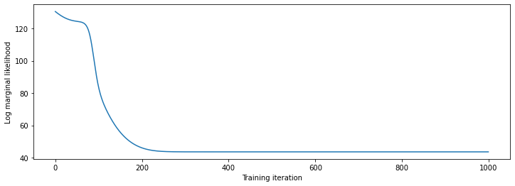
# Plot the loss evolution
plt.figure(figsize=(12, 4))
plt.plot(lls_)
plt.xlabel("Training iteration")
plt.ylabel("Log marginal likelihood")
plt.show()
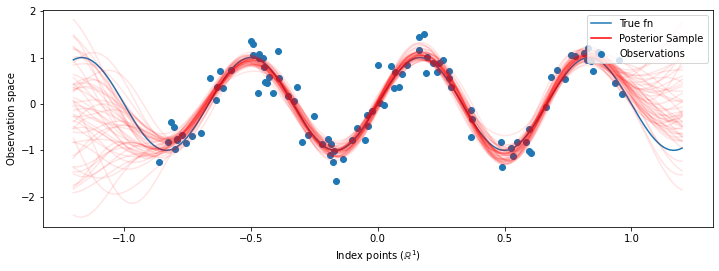
# Having trained the model, we'd like to sample from the posterior conditioned
# on observations. We'd like the samples to be at points other than the training
# inputs.
predictive_index_points_ = np.linspace(-1.2, 1.2, 200, dtype=np.float64)
# Reshape to [200, 1] -- 1 is the dimensionality of the feature space.
predictive_index_points_ = predictive_index_points_[..., np.newaxis]

optimized_kernel = tfk.ExponentiatedQuadratic(amplitude_var, length_scale_var)
gprm = tfd.GaussianProcessRegressionModel(
    kernel=optimized_kernel,
    index_points=predictive_index_points_,
    observation_index_points=observation_index_points_,
    observations=observations_,
    observation_noise_variance=observation_noise_variance_var,
    predictive_noise_variance=0.)

# Create op to draw  50 independent samples, each of which is a *joint* draw
# from the posterior at the predictive_index_points_. Since we have 200 input
# locations as defined above, this posterior distribution over corresponding
# function values is a 200-dimensional multivariate Gaussian distribution!
num_samples = 50
samples = gprm.sample(num_samples)
# Plot the true function, observations, and posterior samples.
plt.figure(figsize=(12, 4))
plt.plot(predictive_index_points_, sinusoid(predictive_index_points_),
         label='True fn')
plt.scatter(observation_index_points_[:, 0], observations_,
            label='Observations')
for i in range(num_samples):
  plt.plot(predictive_index_points_, samples[i, :], c='r', alpha=.1,
           label='Posterior Sample' if i == 0 else None)
leg = plt.legend(loc='upper right')
for lh in leg.legendHandles:
    lh.set_alpha(1)
plt.xlabel(r"Index points ($\mathbb{R}^1$)")
plt.ylabel("Observation space")
plt.show()
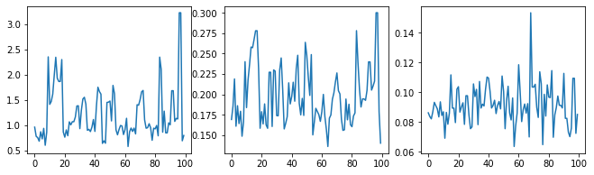
השוליים של היפרפרמטרים עם HMC
במקום לבצע אופטימיזציה של ההיפרפרמטרים, בואו ננסה לשלב אותם עם המילטון מונטה קרלו. תחילה נגדיר ונפעיל דגימה כדי לצייר בערך מההתפלגות האחורית על פני היפרפרמטרים של גרעין, בהתחשב בתצפיות.
num_results = 100
num_burnin_steps = 50

sampler = tfp.mcmc.TransformedTransitionKernel(
    tfp.mcmc.NoUTurnSampler(
        target_log_prob_fn=target_log_prob,
        step_size=tf.cast(0.1, tf.float64)),
    bijector=[constrain_positive, constrain_positive, constrain_positive])

adaptive_sampler = tfp.mcmc.DualAveragingStepSizeAdaptation(
    inner_kernel=sampler,
    num_adaptation_steps=int(0.8 * num_burnin_steps),
    target_accept_prob=tf.cast(0.75, tf.float64))

initial_state = [tf.cast(x, tf.float64) for x in [1., 1., 1.]]
# Speed up sampling by tracing with `tf.function`.
@tf.function(autograph=False, jit_compile=False)
def do_sampling():
  return tfp.mcmc.sample_chain(
      kernel=adaptive_sampler,
      current_state=initial_state,
      num_results=num_results,
      num_burnin_steps=num_burnin_steps,
      trace_fn=lambda current_state, kernel_results: kernel_results)

t0 = time.time()
samples, kernel_results = do_sampling()
t1 = time.time()
print("Inference ran in {:.2f}s.".format(t1-t0))
Inference ran in 9.00s.
בואו נבדוק את הדגימה על-ידי בחינת עקבות ההיפרפרמטרים.
(amplitude_samples,
 length_scale_samples,
 observation_noise_variance_samples) = samples

f = plt.figure(figsize=[15, 3])
for i, s in enumerate(samples):
  ax = f.add_subplot(1, len(samples) + 1, i + 1)
  ax.plot(s)
עכשיו במקום בניית GP יחיד עם hyperparameters אופטימיזציה, אנו בונים את חלוק חזוי האחורית כתערובת של רופאים, כול אחד מהם מוגדר על ידי מדגם מההפצה האחורית מעל hyperparameters. זה משתלב בערך על פני הפרמטרים האחוריים באמצעות דגימת מונטה קרלו כדי לחשב את התפלגות הניבוי השולית במיקומים שלא נצפו.
# The sampled hyperparams have a leading batch dimension, `[num_results, ...]`,
# so they construct a *batch* of kernels.
batch_of_posterior_kernels = tfk.ExponentiatedQuadratic(
    amplitude_samples, length_scale_samples)

# The batch of kernels creates a batch of GP predictive models, one for each
# posterior sample.
batch_gprm = tfd.GaussianProcessRegressionModel(
    kernel=batch_of_posterior_kernels,
    index_points=predictive_index_points_,
    observation_index_points=observation_index_points_,
    observations=observations_,
    observation_noise_variance=observation_noise_variance_samples,
    predictive_noise_variance=0.)

# To construct the marginal predictive distribution, we average with uniform
# weight over the posterior samples.
predictive_gprm = tfd.MixtureSameFamily(
    mixture_distribution=tfd.Categorical(logits=tf.zeros([num_results])),
    components_distribution=batch_gprm)

num_samples = 50
samples = predictive_gprm.sample(num_samples)
# Plot the true function, observations, and posterior samples.
plt.figure(figsize=(12, 4))
plt.plot(predictive_index_points_, sinusoid(predictive_index_points_),
         label='True fn')
plt.scatter(observation_index_points_[:, 0], observations_,
            label='Observations')
for i in range(num_samples):
  plt.plot(predictive_index_points_, samples[i, :], c='r', alpha=.1,
           label='Posterior Sample' if i == 0 else None)
leg = plt.legend(loc='upper right')
for lh in leg.legendHandles:
    lh.set_alpha(1)
plt.xlabel(r"Index points ($\mathbb{R}^1$)")
plt.ylabel("Observation space")
plt.show()
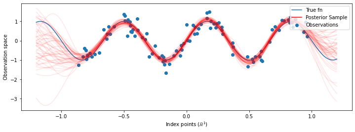
למרות שההבדלים הם עדינים במקרה זה, באופן כללי, היינו מצפים שהתפלגות הניבוי האחורית תכליל טוב יותר (תיתן סבירות גבוהה יותר לנתונים מוחזקים) מאשר רק שימוש בפרמטרים הסבירים ביותר כפי שעשינו למעלה.