| | |  GitHub에서 소스 보기 GitHub에서 소스 보기 |
JointDistributionSequential 새로 도입 분배와 같은 클래스입니다 빠른 프로토 타입 베이지안 모델에 힘을 실어 사용자가. 여러 배포판을 함께 연결하고 람다 함수를 사용하여 종속성을 도입할 수 있습니다. 이것은 GLM, 혼합 효과 모델, 혼합 모델 등과 같이 일반적으로 사용되는 많은 모델을 포함하여 중소 규모 베이지안 모델을 구축하도록 설계되었습니다. 베이지안 워크플로에 필요한 모든 기능을 가능하게 합니다. 사전 예측 샘플링, 다른 더 큰 베이지안 그래픽 모델 또는 신경망에 플러그인할 수 있습니다. 이 Colab에서, 우리는 사용하는 방법에 대한 몇 가지 예를 보여줍니다 JointDistributionSequential 하루 베이지안 워크 플로우 하루를 달성하기 위해
종속성 및 전제 조건
# We will be using ArviZ, a multi-backend Bayesian diagnosis and plotting librarypip3 install -q git+git://github.com/arviz-devs/arviz.git
가져오기 및 설정
from pprint import pprint
import matplotlib.pyplot as plt
import numpy as np
import seaborn as sns
import pandas as pd
import arviz as az

import tensorflow.compat.v2 as tf
tf.enable_v2_behavior()

import tensorflow_probability as tfp

sns.reset_defaults()
#sns.set_style('whitegrid')
#sns.set_context('talk')
sns.set_context(context='talk',font_scale=0.7)

%config InlineBackend.figure_format = 'retina'
%matplotlib inline

tfd = tfp.distributions
tfb = tfp.bijectors

dtype = tf.float64
일을 빨리 만드십시오!
본격적으로 시작하기 전에 이 데모에 GPU를 사용하고 있는지 확인하겠습니다.
이렇게 하려면 "런타임" -> "런타임 유형 변경" -> "하드웨어 가속기" -> "GPU"를 선택합니다.
다음 스니펫은 GPU에 대한 액세스 권한이 있는지 확인합니다.
if tf.test.gpu_device_name() != '/device:GPU:0':
  print('WARNING: GPU device not found.')
else:
  print('SUCCESS: Found GPU: {}'.format(tf.test.gpu_device_name()))
SUCCESS: Found GPU: /device:GPU:0
공동분포
참고: 이 배포 클래스는 간단한 모델만 있는 경우에 유용합니다. "단순"은 사슬 모양의 그래프를 의미합니다. 이 접근 방식은 기술적으로 단일 노드에 대해 최대 255 정도의 모든 PGM에서 작동하지만(파이썬 함수는 최대 이 정도의 인수를 가질 수 있기 때문입니다).
기본적인 아이디어는 사용자의 목록을 지정하는 것입니다 callable 생산의 tfp.Distribution 경우, 자신의 모든 정점에 대해 하나의 PGM을 . callable 목록에서 인덱스 많은 인수로 기껏해야합니다. (사용자 편의를 위해 aguments는 생성의 역순으로 전달됩니다.) 내부적으로는 모든 이전 RV의 값을 각 호출 가능에 전달하여 단순히 "그래프를 탐색"할 것입니다. : 이렇게 우리는 [확률의 체인 룰 (https://en.wikipedia.org/wiki/Chain 규칙 (29 % 확률 # More_than_two_random_variables) 구현 \(p(\{x\}_i^d)=\prod_i^d p(x_i|x_{<i})\).
아이디어는 Python 코드와 마찬가지로 매우 간단합니다. 요지는 다음과 같습니다.
# The chain rule of probability, manifest as Python code.
def log_prob(rvs, xs):
  # xs[:i] is rv[i]'s markov blanket. `[::-1]` just reverses the list.
  return sum(rv(*xs[i-1::-1]).log_prob(xs[i])
             for i, rv in enumerate(rvs))
당신의 문서화 문자열에서 더 많은 정보를 찾을 수 있습니다 JointDistributionSequential 하지만, 요점은 당신이 클래스를 초기화하는 배포판의 목록을 통과한다는 것입니다 목록의 일부 분포가 다른 업스트림 유통 / 가변 출력에 따라 경우, 당신은 단지 그것을 포장 람다 함수. 이제 어떻게 작동하는지 봅시다!
(강력한) 선형 회귀
PyMC3의 문서의에서 GLM : 특이점 탐지와 강력한 회귀
데이터 가져오기
dfhogg = pd.DataFrame(np.array([[1, 201, 592, 61, 9, -0.84],
[2, 244, 401, 25, 4, 0.31],
[3, 47, 583, 38, 11, 0.64],
[4, 287, 402, 15, 7, -0.27],
[5, 203, 495, 21, 5, -0.33],
[6, 58, 173, 15, 9, 0.67],
[7, 210, 479, 27, 4, -0.02],
[8, 202, 504, 14, 4, -0.05],
[9, 198, 510, 30, 11, -0.84],
[10, 158, 416, 16, 7, -0.69],
[11, 165, 393, 14, 5, 0.30],
[12, 201, 442, 25, 5, -0.46],
[13, 157, 317, 52, 5, -0.03],
[14, 131, 311, 16, 6, 0.50],
[15, 166, 400, 34, 6, 0.73],
[16, 160, 337, 31, 5, -0.52],
[17, 186, 423, 42, 9, 0.90],
[18, 125, 334, 26, 8, 0.40],
[19, 218, 533, 16, 6, -0.78],
[20, 146, 344, 22, 5, -0.56]]),
columns=['id','x','y','sigma_y','sigma_x','rho_xy'])
## for convenience zero-base the 'id' and use as index
dfhogg['id'] = dfhogg['id'] - 1
dfhogg.set_index('id', inplace=True)
## standardize (mean center and divide by 1 sd)
dfhoggs = (dfhogg[['x','y']] - dfhogg[['x','y']].mean(0)) / dfhogg[['x','y']].std(0)
dfhoggs['sigma_y'] = dfhogg['sigma_y'] / dfhogg['y'].std(0)
dfhoggs['sigma_x'] = dfhogg['sigma_x'] / dfhogg['x'].std(0)
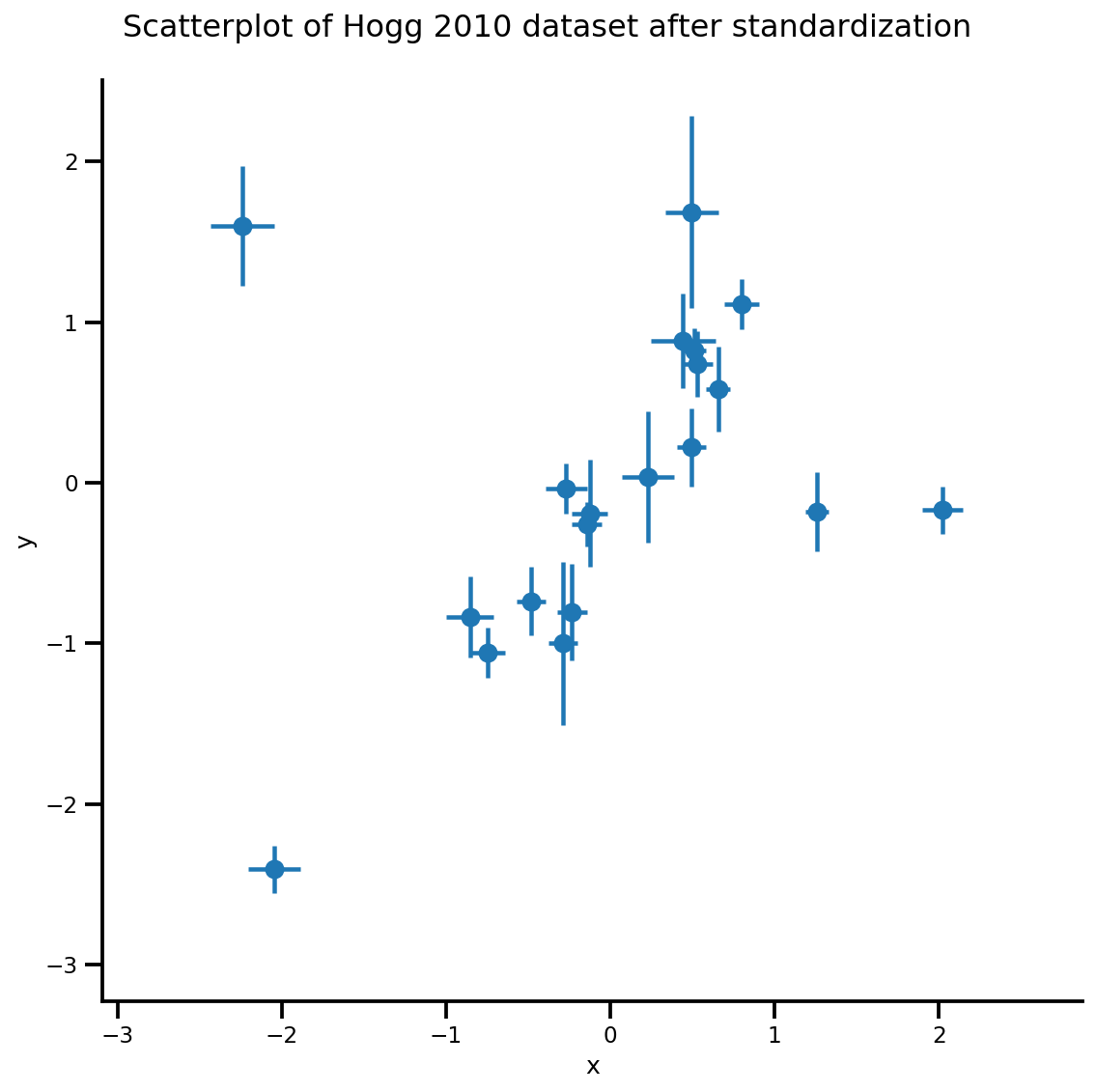
def plot_hoggs(dfhoggs):
## create xlims ylims for plotting
xlims = (dfhoggs['x'].min() - np.ptp(dfhoggs['x'])/5,
dfhoggs['x'].max() + np.ptp(dfhoggs['x'])/5)
ylims = (dfhoggs['y'].min() - np.ptp(dfhoggs['y'])/5,
dfhoggs['y'].max() + np.ptp(dfhoggs['y'])/5)
## scatterplot the standardized data
g = sns.FacetGrid(dfhoggs, size=8)
_ = g.map(plt.errorbar, 'x', 'y', 'sigma_y', 'sigma_x', marker="o", ls='')
_ = g.axes[0][0].set_ylim(ylims)
_ = g.axes[0][0].set_xlim(xlims)
plt.subplots_adjust(top=0.92)
_ = g.fig.suptitle('Scatterplot of Hogg 2010 dataset after standardization', fontsize=16)
return g, xlims, ylims
g = plot_hoggs(dfhoggs)
/usr/local/lib/python3.6/dist-packages/numpy/core/fromnumeric.py:2495: FutureWarning: Method .ptp is deprecated and will be removed in a future version. Use numpy.ptp instead.
  return ptp(axis=axis, out=out, **kwargs)
/usr/local/lib/python3.6/dist-packages/seaborn/axisgrid.py:230: UserWarning: The `size` paramter has been renamed to `height`; please update your code.
  warnings.warn(msg, UserWarning)
X_np = dfhoggs['x'].values
sigma_y_np = dfhoggs['sigma_y'].values
Y_np = dfhoggs['y'].values
기존 OLS 모델
이제 간단한 절편 + 기울기 회귀 문제인 선형 모델을 설정해 보겠습니다.
mdl_ols = tfd.JointDistributionSequential([
    # b0 ~ Normal(0, 1)
    tfd.Normal(loc=tf.cast(0, dtype), scale=1.),
    # b1 ~ Normal(0, 1)
    tfd.Normal(loc=tf.cast(0, dtype), scale=1.),
    # x ~ Normal(b0+b1*X, 1)
    lambda b1, b0: tfd.Normal(
      # Parameter transformation
      loc=b0 + b1*X_np,
      scale=sigma_y_np)
])
그런 다음 모델의 그래프를 확인하여 종속성을 확인할 수 있습니다. 참고 x 마지막 노드의 이름으로 예약되어, 당신은 확실하지 그것을 당신의 JointDistributionSequential 모델에 람다 인수로 할 수 있습니다.
mdl_ols.resolve_graph()
(('b0', ()), ('b1', ()), ('x', ('b1', 'b0')))
모델에서 샘플링하는 것은 매우 간단합니다.
mdl_ols.sample()
[<tf.Tensor: shape=(), dtype=float64, numpy=-0.50225804634794>,
 <tf.Tensor: shape=(), dtype=float64, numpy=0.682740126293564>,
 <tf.Tensor: shape=(20,), dtype=float64, numpy=
 array([-0.33051382,  0.71443618, -1.91085683,  0.89371173, -0.45060957,
        -1.80448758, -0.21357082,  0.07891058, -0.20689721, -0.62690385,
        -0.55225748, -0.11446535, -0.66624497, -0.86913291, -0.93605552,
        -0.83965336, -0.70988597, -0.95813437,  0.15884761, -0.31113434])>]
...tf.Tensor의 목록을 제공합니다. 즉시 log_prob 함수에 연결하여 모델의 log_prob를 계산할 수 있습니다.
prior_predictive_samples = mdl_ols.sample()
mdl_ols.log_prob(prior_predictive_samples)
<tf.Tensor: shape=(20,), dtype=float64, numpy=
array([-4.97502846, -3.98544303, -4.37514505, -3.46933487, -3.80688125,
       -3.42907525, -4.03263074, -3.3646366 , -4.70370938, -4.36178501,
       -3.47823735, -3.94641662, -5.76906319, -4.0944128 , -4.39310708,
       -4.47713894, -4.46307881, -3.98802372, -3.83027747, -4.64777082])>
흠, 뭔가 잘못되었습니다. 스칼라 log_prob를 얻어야 합니다! 사실, 우리는 더 뭔가를 호출하여 꺼져 있는지 확인할 수 있습니다 .log_prob_parts 제공, log_prob 그래픽 모델의 각 노드를 :
mdl_ols.log_prob_parts(prior_predictive_samples)
[<tf.Tensor: shape=(), dtype=float64, numpy=-0.9699239562734849>,
 <tf.Tensor: shape=(), dtype=float64, numpy=-3.459364167569284>,
 <tf.Tensor: shape=(20,), dtype=float64, numpy=
 array([-0.54574034,  0.4438451 ,  0.05414307,  0.95995326,  0.62240687,
         1.00021288,  0.39665739,  1.06465152, -0.27442125,  0.06750311,
         0.95105078,  0.4828715 , -1.33977506,  0.33487533,  0.03618104,
        -0.04785082, -0.03379069,  0.4412644 ,  0.59901066, -0.2184827 ])>]
...마지막 노드가 iid 차원/축을 따라 reduce_sum이 아닌 것으로 나타났습니다! 합을 할 때 처음 두 변수는 잘못 브로드캐스트됩니다.
여기에 트릭은 사용하는 것입니다 tfd.Independent 배치 형태 (그래서 축의 나머지가 제대로 감소됩니다) 재 해석에 :
mdl_ols_ = tfd.JointDistributionSequential([
    # b0
    tfd.Normal(loc=tf.cast(0, dtype), scale=1.),
    # b1
    tfd.Normal(loc=tf.cast(0, dtype), scale=1.),
    # likelihood
    #   Using Independent to ensure the log_prob is not incorrectly broadcasted
    lambda b1, b0: tfd.Independent(
        tfd.Normal(
            # Parameter transformation
            # b1 shape: (batch_shape), X shape (num_obs): we want result to have
            # shape (batch_shape, num_obs)
            loc=b0 + b1*X_np,
            scale=sigma_y_np),
        reinterpreted_batch_ndims=1
    ),
])
이제 모델의 마지막 노드/분포를 확인하겠습니다. 이제 이벤트 모양이 올바르게 해석된 것을 볼 수 있습니다. 참고 그것을 얻기 위해 시행 착오를 조금 걸릴 수 있다는 reinterpreted_batch_ndims 잘하지만, 당신은 항상 쉽게 한 번 확인에 배포 또는 샘플링 텐서 모양을 인쇄 할 수 있습니다!
print(mdl_ols_.sample_distributions()[0][-1])
print(mdl_ols.sample_distributions()[0][-1])
tfp.distributions.Independent("JointDistributionSequential_sample_distributions_IndependentJointDistributionSequential_sample_distributions_Normal", batch_shape=[], event_shape=[20], dtype=float64)
tfp.distributions.Normal("JointDistributionSequential_sample_distributions_Normal", batch_shape=[20], event_shape=[], dtype=float64)
prior_predictive_samples = mdl_ols_.sample()
mdl_ols_.log_prob(prior_predictive_samples)  # <== Getting a scalar correctly
<tf.Tensor: shape=(), dtype=float64, numpy=-2.543425661013286>
다른 JointDistribution* API
mdl_ols_named = tfd.JointDistributionNamed(dict(
    likelihood = lambda b0, b1: tfd.Independent(
        tfd.Normal(
            loc=b0 + b1*X_np,
            scale=sigma_y_np),
        reinterpreted_batch_ndims=1
    ),
    b0         = tfd.Normal(loc=tf.cast(0, dtype), scale=1.),
    b1         = tfd.Normal(loc=tf.cast(0, dtype), scale=1.),
))

mdl_ols_named.log_prob(mdl_ols_named.sample())
<tf.Tensor: shape=(), dtype=float64, numpy=-5.99620966071338>
mdl_ols_named.sample() # output is a dictionary
{'b0': <tf.Tensor: shape=(), dtype=float64, numpy=0.26364058399428225>,
 'b1': <tf.Tensor: shape=(), dtype=float64, numpy=-0.27209402374432207>,
 'likelihood': <tf.Tensor: shape=(20,), dtype=float64, numpy=
 array([ 0.6482155 , -0.39314108,  0.62744764, -0.24587987, -0.20544617,
         1.01465392, -0.04705611, -0.16618702,  0.36410134,  0.3943299 ,
         0.36455291, -0.27822219, -0.24423928,  0.24599518,  0.82731092,
        -0.21983033,  0.56753169,  0.32830481, -0.15713064,  0.23336351])>}
Root = tfd.JointDistributionCoroutine.Root  # Convenient alias.
def model():
  b1 = yield Root(tfd.Normal(loc=tf.cast(0, dtype), scale=1.))
  b0 = yield Root(tfd.Normal(loc=tf.cast(0, dtype), scale=1.))
  yhat = b0 + b1*X_np
  likelihood = yield tfd.Independent(
        tfd.Normal(loc=yhat, scale=sigma_y_np),
        reinterpreted_batch_ndims=1
    )

mdl_ols_coroutine = tfd.JointDistributionCoroutine(model)
mdl_ols_coroutine.log_prob(mdl_ols_coroutine.sample())
<tf.Tensor: shape=(), dtype=float64, numpy=-4.566678123520463>
mdl_ols_coroutine.sample() # output is a tuple
(<tf.Tensor: shape=(), dtype=float64, numpy=0.06811002171170354>,
 <tf.Tensor: shape=(), dtype=float64, numpy=-0.37477064754116807>,
 <tf.Tensor: shape=(20,), dtype=float64, numpy=
 array([-0.91615096, -0.20244718, -0.47840159, -0.26632479, -0.60441105,
        -0.48977789, -0.32422329, -0.44019322, -0.17072643, -0.20666025,
        -0.55932191, -0.40801868, -0.66893181, -0.24134135, -0.50403536,
        -0.51788596, -0.90071876, -0.47382338, -0.34821655, -0.38559724])>)
MLE
이제 추론을 할 수 있습니다! 옵티마이저를 사용하여 최대 우도 추정을 찾을 수 있습니다.
일부 도우미 함수 정의
# bfgs and lbfgs currently requries a function that returns both the value and
# gradient re the input.
import functools

def _make_val_and_grad_fn(value_fn):
  @functools.wraps(value_fn)
  def val_and_grad(x):
    return tfp.math.value_and_gradient(value_fn, x)
  return val_and_grad

# Map a list of tensors (e.g., output from JDSeq.sample([...])) to a single tensor
# modify from tfd.Blockwise
from tensorflow_probability.python.internal import dtype_util
from tensorflow_probability.python.internal import prefer_static as ps
from tensorflow_probability.python.internal import tensorshape_util

class Mapper:
  """Basically, this is a bijector without log-jacobian correction."""
  def __init__(self, list_of_tensors, list_of_bijectors, event_shape):
    self.dtype = dtype_util.common_dtype(
        list_of_tensors, dtype_hint=tf.float32)
    self.list_of_tensors = list_of_tensors
    self.bijectors = list_of_bijectors
    self.event_shape = event_shape

  def flatten_and_concat(self, list_of_tensors):
    def _reshape_map_part(part, event_shape, bijector):
      part = tf.cast(bijector.inverse(part), self.dtype)
      static_rank = tf.get_static_value(ps.rank_from_shape(event_shape))
      if static_rank == 1:
        return part
      new_shape = ps.concat([
          ps.shape(part)[:ps.size(ps.shape(part)) - ps.size(event_shape)],
          [-1]
      ], axis=-1)
      return tf.reshape(part, ps.cast(new_shape, tf.int32))

    x = tf.nest.map_structure(_reshape_map_part,
                              list_of_tensors,
                              self.event_shape,
                              self.bijectors)
    return tf.concat(tf.nest.flatten(x), axis=-1)

  def split_and_reshape(self, x):
    assertions = []
    message = 'Input must have at least one dimension.'
    if tensorshape_util.rank(x.shape) is not None:
      if tensorshape_util.rank(x.shape) == 0:
        raise ValueError(message)
    else:
      assertions.append(assert_util.assert_rank_at_least(x, 1, message=message))
    with tf.control_dependencies(assertions):
      splits = [
          tf.cast(ps.maximum(1, ps.reduce_prod(s)), tf.int32)
          for s in tf.nest.flatten(self.event_shape)
      ]
      x = tf.nest.pack_sequence_as(
          self.event_shape, tf.split(x, splits, axis=-1))
      def _reshape_map_part(part, part_org, event_shape, bijector):
        part = tf.cast(bijector.forward(part), part_org.dtype)
        static_rank = tf.get_static_value(ps.rank_from_shape(event_shape))
        if static_rank == 1:
          return part
        new_shape = ps.concat([ps.shape(part)[:-1], event_shape], axis=-1)
        return tf.reshape(part, ps.cast(new_shape, tf.int32))

      x = tf.nest.map_structure(_reshape_map_part,
                                x,
                                self.list_of_tensors,
                                self.event_shape,
                                self.bijectors)
    return x
mapper = Mapper(mdl_ols_.sample()[:-1],
                [tfb.Identity(), tfb.Identity()],
                mdl_ols_.event_shape[:-1])

# mapper.split_and_reshape(mapper.flatten_and_concat(mdl_ols_.sample()[:-1]))
@_make_val_and_grad_fn
def neg_log_likelihood(x):
  # Generate a function closure so that we are computing the log_prob
  # conditioned on the observed data. Note also that tfp.optimizer.* takes a
  # single tensor as input.
  return -mdl_ols_.log_prob(mapper.split_and_reshape(x) + [Y_np])

lbfgs_results = tfp.optimizer.lbfgs_minimize(
    neg_log_likelihood,
    initial_position=tf.zeros(2, dtype=dtype),
    tolerance=1e-20,
    x_tolerance=1e-8
)
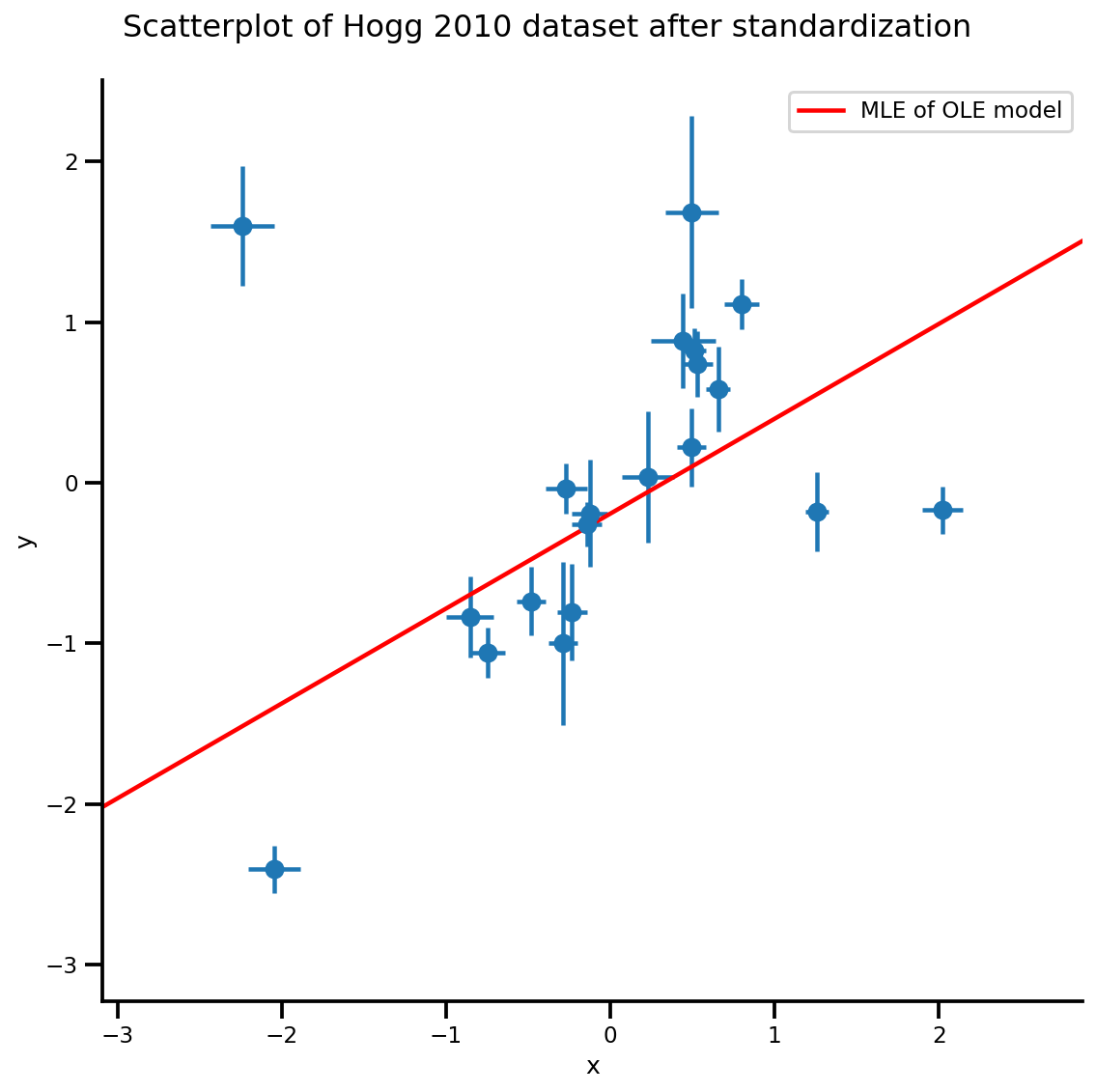
b0est, b1est = lbfgs_results.position.numpy()

g, xlims, ylims = plot_hoggs(dfhoggs);
xrange = np.linspace(xlims[0], xlims[1], 100)
g.axes[0][0].plot(xrange, b0est + b1est*xrange,
                  color='r', label='MLE of OLE model')
plt.legend();
/usr/local/lib/python3.6/dist-packages/numpy/core/fromnumeric.py:2495: FutureWarning: Method .ptp is deprecated and will be removed in a future version. Use numpy.ptp instead.
  return ptp(axis=axis, out=out, **kwargs)
/usr/local/lib/python3.6/dist-packages/seaborn/axisgrid.py:230: UserWarning: The `size` paramter has been renamed to `height`; please update your code.
  warnings.warn(msg, UserWarning)
일괄 버전 모델 및 MCMC
샘플이 후방에서 때, 우리는 컴퓨팅의 기대에 대한 함수로 그들을 연결 수 베이지안 추론에서, 우리는 일반적으로, MCMC 샘플 작업 할. 그러나, MCMC API가 배치 친화적 인 모델을 작성하는 우리를 필요로하며, 우리가 우리의 모델을 호출하여 실제로 "batchable"아님을 확인하실 수 있습니다 sample([...])
mdl_ols_.sample(5) # <== error as some computation could not be broadcasted.
이 경우 모델 내부에 선형 함수만 있기 때문에 비교적 간단합니다. 모양을 확장하면 트릭을 수행해야 합니다.
mdl_ols_batch = tfd.JointDistributionSequential([
    # b0
    tfd.Normal(loc=tf.cast(0, dtype), scale=1.),
    # b1
    tfd.Normal(loc=tf.cast(0, dtype), scale=1.),
    # likelihood
    #   Using Independent to ensure the log_prob is not incorrectly broadcasted
    lambda b1, b0: tfd.Independent(
        tfd.Normal(
            # Parameter transformation
            loc=b0[..., tf.newaxis] + b1[..., tf.newaxis]*X_np[tf.newaxis, ...],
            scale=sigma_y_np[tf.newaxis, ...]),
        reinterpreted_batch_ndims=1
    ),
])

mdl_ols_batch.resolve_graph()
(('b0', ()), ('b1', ()), ('x', ('b1', 'b0')))
몇 가지 검사를 수행하기 위해 log_prob_parts를 다시 샘플링하고 평가할 수 있습니다.
b0, b1, y = mdl_ols_batch.sample(4)
mdl_ols_batch.log_prob_parts([b0, b1, y])
[<tf.Tensor: shape=(4,), dtype=float64, numpy=array([-1.25230168, -1.45281432, -1.87110061, -1.07665206])>,
 <tf.Tensor: shape=(4,), dtype=float64, numpy=array([-1.07019936, -1.59562117, -2.53387765, -1.01557632])>,
 <tf.Tensor: shape=(4,), dtype=float64, numpy=array([ 0.45841406,  2.56829635, -4.84973951, -5.59423992])>]
몇 가지 참고 사항:
- 다중 체인 MCMC에서 가장 빠르기 때문에 모델의 배치 버전으로 작업하고 싶습니다. 당신이 일괄 버전 (예를 들어, ODE 모델)과 같은 모델을 다시 작성할 수없는 경우에, 당신은 사용 log_prob 기능을 매핑 할 수 있습니다
tf.map_fn동일한 효과를 얻을 수 있습니다. - 이제
mdl_ols_batch.sample()우리가 할 수 없기 때문에 우리는 스케일러 이전하지 작업을해야 할 수도 있습니다으로scaler_tensor[:, None]. 여기서 용액 배치하여 순위 1 스케일러 텐서 확장하는tfd.Sample(..., sample_shape=1). - 하이퍼파라미터와 같은 설정을 훨씬 쉽게 변경할 수 있도록 모델을 함수로 작성하는 것이 좋습니다.
def gen_ols_batch_model(X, sigma, hyperprior_mean=0, hyperprior_scale=1):
  hyper_mean = tf.cast(hyperprior_mean, dtype)
  hyper_scale = tf.cast(hyperprior_scale, dtype)
  return tfd.JointDistributionSequential([
      # b0
      tfd.Sample(tfd.Normal(loc=hyper_mean, scale=hyper_scale), sample_shape=1),
      # b1
      tfd.Sample(tfd.Normal(loc=hyper_mean, scale=hyper_scale), sample_shape=1),
      # likelihood
      lambda b1, b0: tfd.Independent(
          tfd.Normal(
              # Parameter transformation
              loc=b0 + b1*X,
              scale=sigma),
          reinterpreted_batch_ndims=1
      ),
  ], validate_args=True)

mdl_ols_batch = gen_ols_batch_model(X_np[tf.newaxis, ...],
                                    sigma_y_np[tf.newaxis, ...])

_ = mdl_ols_batch.sample()
_ = mdl_ols_batch.sample(4)
_ = mdl_ols_batch.sample([3, 4])
# Small helper function to validate log_prob shape (avoid wrong broadcasting)
def validate_log_prob_part(model, batch_shape=1, observed=-1):
  samples = model.sample(batch_shape)
  logp_part = list(model.log_prob_parts(samples))

  # exclude observed node
  logp_part.pop(observed)
  for part in logp_part:
    tf.assert_equal(part.shape, logp_part[-1].shape)

validate_log_prob_part(mdl_ols_batch, 4)
추가 검사: 생성된 log_prob 함수를 손으로 쓴 TFP log_prob 함수와 비교합니다.
def ols_logp_batch(b0, b1, Y):
  b0_prior = tfd.Normal(loc=tf.cast(0, dtype), scale=1.) # b0
  b1_prior = tfd.Normal(loc=tf.cast(0, dtype), scale=1.) # b1
  likelihood = tfd.Normal(loc=b0 + b1*X_np[None, :],
                          scale=sigma_y_np) # likelihood
  return tf.reduce_sum(b0_prior.log_prob(b0), axis=-1) +\
         tf.reduce_sum(b1_prior.log_prob(b1), axis=-1) +\
         tf.reduce_sum(likelihood.log_prob(Y), axis=-1)

b0, b1, x = mdl_ols_batch.sample(4)
print(mdl_ols_batch.log_prob([b0, b1, Y_np]).numpy())
print(ols_logp_batch(b0, b1, Y_np).numpy())
[-227.37899384 -327.10043743 -570.44162789 -702.79808683]
[-227.37899384 -327.10043743 -570.44162789 -702.79808683]
No-U-Turn Sampler를 사용하는 MCMC
일반적인 run_chain 기능
@tf.function(autograph=False, experimental_compile=True)
def run_chain(init_state, step_size, target_log_prob_fn, unconstraining_bijectors,
              num_steps=500, burnin=50):

  def trace_fn(_, pkr):
    return (
        pkr.inner_results.inner_results.target_log_prob,
        pkr.inner_results.inner_results.leapfrogs_taken,
        pkr.inner_results.inner_results.has_divergence,
        pkr.inner_results.inner_results.energy,
        pkr.inner_results.inner_results.log_accept_ratio
           )

  kernel = tfp.mcmc.TransformedTransitionKernel(
    inner_kernel=tfp.mcmc.NoUTurnSampler(
      target_log_prob_fn,
      step_size=step_size),
    bijector=unconstraining_bijectors)

  hmc = tfp.mcmc.DualAveragingStepSizeAdaptation(
    inner_kernel=kernel,
    num_adaptation_steps=burnin,
    step_size_setter_fn=lambda pkr, new_step_size: pkr._replace(
        inner_results=pkr.inner_results._replace(step_size=new_step_size)),
    step_size_getter_fn=lambda pkr: pkr.inner_results.step_size,
    log_accept_prob_getter_fn=lambda pkr: pkr.inner_results.log_accept_ratio
  )

  # Sampling from the chain.
  chain_state, sampler_stat = tfp.mcmc.sample_chain(
      num_results=num_steps,
      num_burnin_steps=burnin,
      current_state=init_state,
      kernel=hmc,
      trace_fn=trace_fn)
  return chain_state, sampler_stat
nchain = 10
b0, b1, _ = mdl_ols_batch.sample(nchain)
init_state = [b0, b1]
step_size = [tf.cast(i, dtype=dtype) for i in [.1, .1]]
target_log_prob_fn = lambda *x: mdl_ols_batch.log_prob(x + (Y_np, ))

# bijector to map contrained parameters to real
unconstraining_bijectors = [
    tfb.Identity(),
    tfb.Identity(),
]

samples, sampler_stat = run_chain(
    init_state, step_size, target_log_prob_fn, unconstraining_bijectors)
# using the pymc3 naming convention
sample_stats_name = ['lp', 'tree_size', 'diverging', 'energy', 'mean_tree_accept']
sample_stats = {k:v.numpy().T for k, v in zip(sample_stats_name, sampler_stat)}
sample_stats['tree_size'] = np.diff(sample_stats['tree_size'], axis=1)
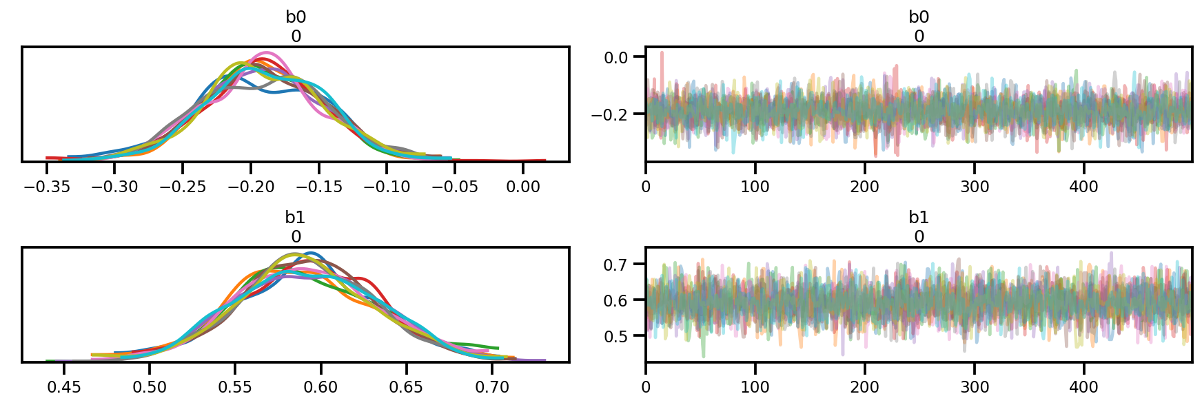
var_name = ['b0', 'b1']
posterior = {k:np.swapaxes(v.numpy(), 1, 0)
for k, v in zip(var_name, samples)}
az_trace = az.from_dict(posterior=posterior, sample_stats=sample_stats)
az.plot_trace(az_trace);
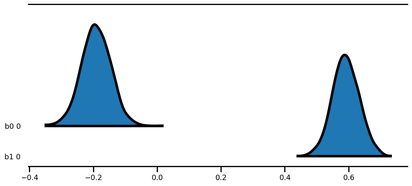
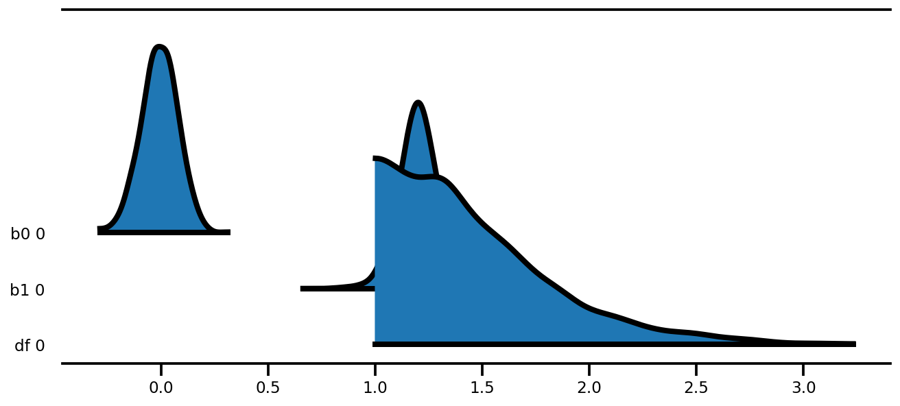
az.plot_forest(az_trace,
               kind='ridgeplot',
               linewidth=4,
               combined=True,
               ridgeplot_overlap=1.5,
               figsize=(9, 4));
k = 5
b0est, b1est = az_trace.posterior['b0'][:, -k:].values, az_trace.posterior['b1'][:, -k:].values
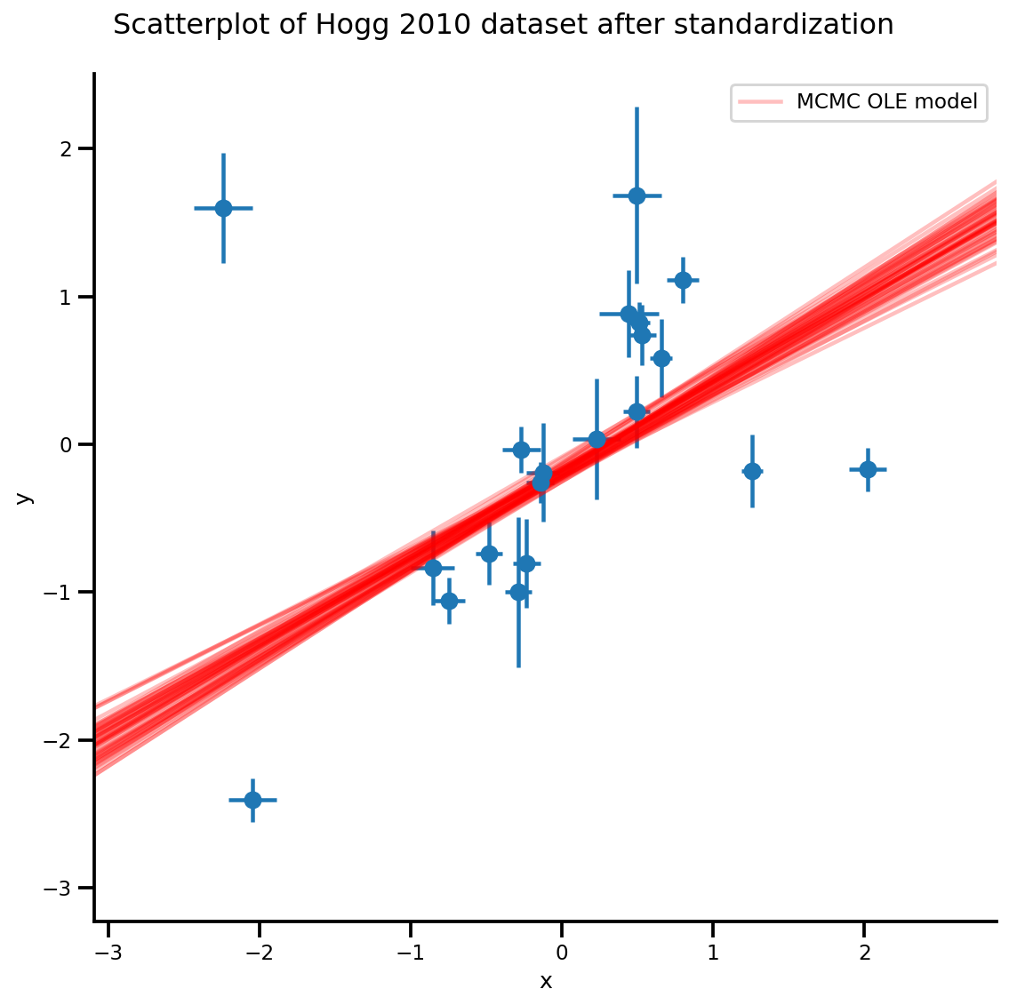
g, xlims, ylims = plot_hoggs(dfhoggs);
xrange = np.linspace(xlims[0], xlims[1], 100)[None, :]
g.axes[0][0].plot(np.tile(xrange, (k, 1)).T,
(np.reshape(b0est, [-1, 1]) + np.reshape(b1est, [-1, 1])*xrange).T,
alpha=.25, color='r')
plt.legend([g.axes[0][0].lines[-1]], ['MCMC OLE model']);
/usr/local/lib/python3.6/dist-packages/numpy/core/fromnumeric.py:2495: FutureWarning: Method .ptp is deprecated and will be removed in a future version. Use numpy.ptp instead.
  return ptp(axis=axis, out=out, **kwargs)
/usr/local/lib/python3.6/dist-packages/seaborn/axisgrid.py:230: UserWarning: The `size` paramter has been renamed to `height`; please update your code.
  warnings.warn(msg, UserWarning)
/usr/local/lib/python3.6/dist-packages/ipykernel_launcher.py:8: MatplotlibDeprecationWarning: cycling among columns of inputs with non-matching shapes is deprecated.
스튜던트-T 방법
지금부터 우리는 항상 모델의 배치 버전으로 작업합니다.
def gen_studentt_model(X, sigma,
                       hyper_mean=0, hyper_scale=1, lower=1, upper=100):
  loc = tf.cast(hyper_mean, dtype)
  scale = tf.cast(hyper_scale, dtype)
  low = tf.cast(lower, dtype)
  high = tf.cast(upper, dtype)
  return tfd.JointDistributionSequential([
      # b0 ~ Normal(0, 1)
      tfd.Sample(tfd.Normal(loc, scale), sample_shape=1),
      # b1 ~ Normal(0, 1)
      tfd.Sample(tfd.Normal(loc, scale), sample_shape=1),
      # df ~ Uniform(a, b)
      tfd.Sample(tfd.Uniform(low, high), sample_shape=1),
      # likelihood ~ StudentT(df, f(b0, b1), sigma_y)
      #   Using Independent to ensure the log_prob is not incorrectly broadcasted.
      lambda df, b1, b0: tfd.Independent(
          tfd.StudentT(df=df, loc=b0 + b1*X, scale=sigma)),
  ], validate_args=True)

mdl_studentt = gen_studentt_model(X_np[tf.newaxis, ...],
                                  sigma_y_np[tf.newaxis, ...])
mdl_studentt.resolve_graph()
(('b0', ()), ('b1', ()), ('df', ()), ('x', ('df', 'b1', 'b0')))
validate_log_prob_part(mdl_studentt, 4)
순방향 표본(사전 예측 표본 추출)
b0, b1, df, x = mdl_studentt.sample(1000)
x.shape
TensorShape([1000, 20])
MLE
# bijector to map contrained parameters to real
a, b = tf.constant(1., dtype), tf.constant(100., dtype),

# Interval transformation
tfp_interval = tfb.Inline(
    inverse_fn=(
        lambda x: tf.math.log(x - a) - tf.math.log(b - x)),
    forward_fn=(
        lambda y: (b - a) * tf.sigmoid(y) + a),
    forward_log_det_jacobian_fn=(
        lambda x: tf.math.log(b - a) - 2 * tf.nn.softplus(-x) - x),
    forward_min_event_ndims=0,
    name="interval")

unconstraining_bijectors = [
    tfb.Identity(),
    tfb.Identity(),
    tfp_interval,
]

mapper = Mapper(mdl_studentt.sample()[:-1],
                unconstraining_bijectors,
                mdl_studentt.event_shape[:-1])
@_make_val_and_grad_fn
def neg_log_likelihood(x):
  # Generate a function closure so that we are computing the log_prob
  # conditioned on the observed data. Note also that tfp.optimizer.* takes a
  # single tensor as input, so we need to do some slicing here:
  return -tf.squeeze(mdl_studentt.log_prob(
      mapper.split_and_reshape(x) + [Y_np]))

lbfgs_results = tfp.optimizer.lbfgs_minimize(
    neg_log_likelihood,
    initial_position=mapper.flatten_and_concat(mdl_studentt.sample()[:-1]),
    tolerance=1e-20,
    x_tolerance=1e-20
)
b0est, b1est, dfest = lbfgs_results.position.numpy()
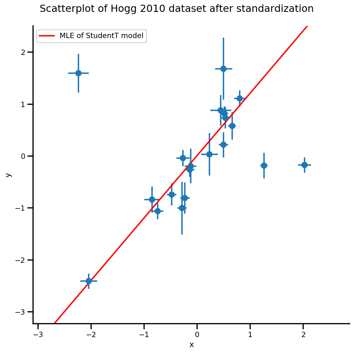
g, xlims, ylims = plot_hoggs(dfhoggs);
xrange = np.linspace(xlims[0], xlims[1], 100)
g.axes[0][0].plot(xrange, b0est + b1est*xrange,
color='r', label='MLE of StudentT model')
plt.legend();
/usr/local/lib/python3.6/dist-packages/numpy/core/fromnumeric.py:2495: FutureWarning: Method .ptp is deprecated and will be removed in a future version. Use numpy.ptp instead.
  return ptp(axis=axis, out=out, **kwargs)
/usr/local/lib/python3.6/dist-packages/seaborn/axisgrid.py:230: UserWarning: The `size` paramter has been renamed to `height`; please update your code.
  warnings.warn(msg, UserWarning)
MCMC
nchain = 10
b0, b1, df, _ = mdl_studentt.sample(nchain)
init_state = [b0, b1, df]
step_size = [tf.cast(i, dtype=dtype) for i in [.1, .1, .05]]

target_log_prob_fn = lambda *x: mdl_studentt.log_prob(x + (Y_np, ))

samples, sampler_stat = run_chain(
    init_state, step_size, target_log_prob_fn, unconstraining_bijectors, burnin=100)
# using the pymc3 naming convention
sample_stats_name = ['lp', 'tree_size', 'diverging', 'energy', 'mean_tree_accept']
sample_stats = {k:v.numpy().T for k, v in zip(sample_stats_name, sampler_stat)}
sample_stats['tree_size'] = np.diff(sample_stats['tree_size'], axis=1)
var_name = ['b0', 'b1', 'df']
posterior = {k:np.swapaxes(v.numpy(), 1, 0)
for k, v in zip(var_name, samples)}
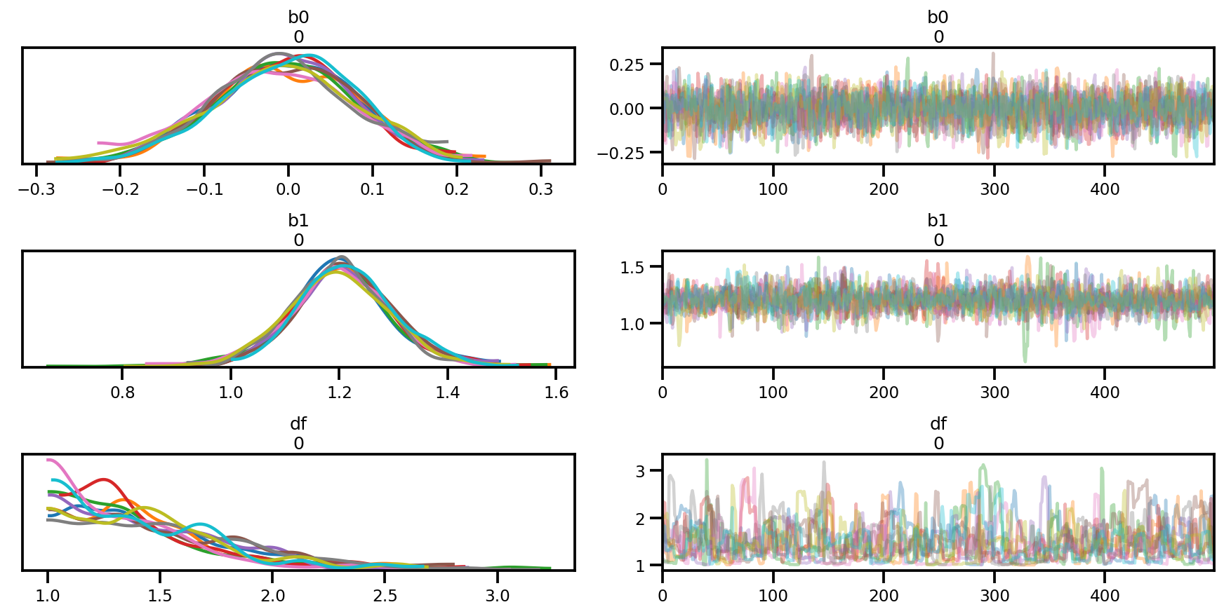
az_trace = az.from_dict(posterior=posterior, sample_stats=sample_stats)
az.summary(az_trace)
az.plot_trace(az_trace);
az.plot_forest(az_trace,
               kind='ridgeplot',
               linewidth=4,
               combined=True,
               ridgeplot_overlap=1.5,
               figsize=(9, 4));
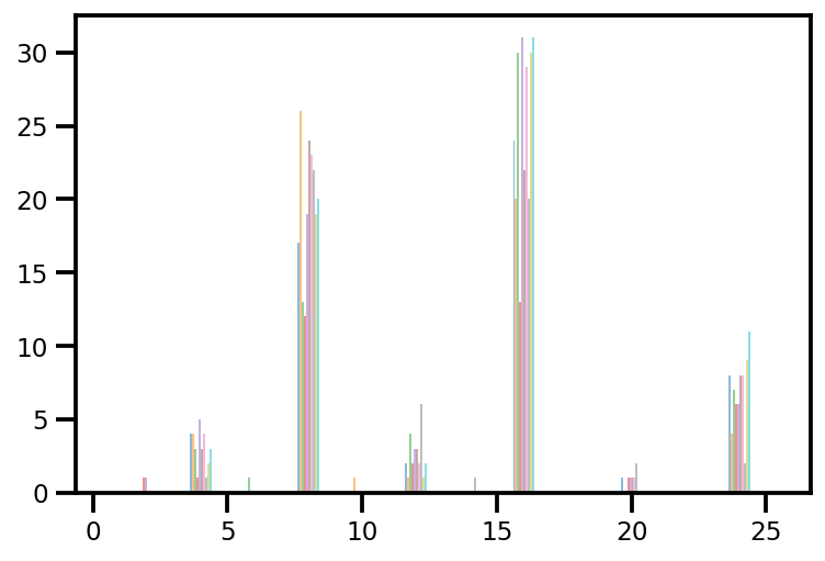
plt.hist(az_trace.sample_stats['tree_size'], np.linspace(.5, 25.5, 26), alpha=.5);
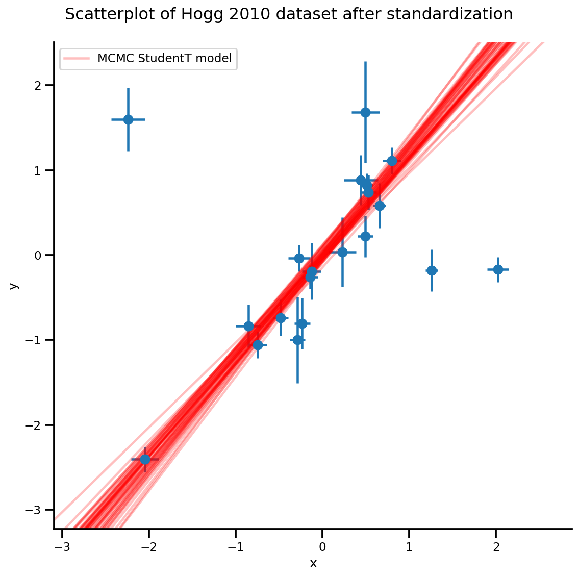
k = 5
b0est, b1est = az_trace.posterior['b0'][:, -k:].values, az_trace.posterior['b1'][:, -k:].values

g, xlims, ylims = plot_hoggs(dfhoggs);
xrange = np.linspace(xlims[0], xlims[1], 100)[None, :]
g.axes[0][0].plot(np.tile(xrange, (k, 1)).T,
                  (np.reshape(b0est, [-1, 1]) + np.reshape(b1est, [-1, 1])*xrange).T,
                  alpha=.25, color='r')
plt.legend([g.axes[0][0].lines[-1]], ['MCMC StudentT model']);
/usr/local/lib/python3.6/dist-packages/numpy/core/fromnumeric.py:2495: FutureWarning: Method .ptp is deprecated and will be removed in a future version. Use numpy.ptp instead.
  return ptp(axis=axis, out=out, **kwargs)
/usr/local/lib/python3.6/dist-packages/seaborn/axisgrid.py:230: UserWarning: The `size` paramter has been renamed to `height`; please update your code.
  warnings.warn(msg, UserWarning)
/usr/local/lib/python3.6/dist-packages/ipykernel_launcher.py:8: MatplotlibDeprecationWarning: cycling among columns of inputs with non-matching shapes is deprecated.
계층적 부분 풀링
PyMC3의에서 에프론과 모리스 18 명 선수 야구 데이터 (1975)
data = pd.read_table('https://raw.githubusercontent.com/pymc-devs/pymc3/master/pymc3/examples/data/efron-morris-75-data.tsv',
                     sep="\t")
at_bats, hits = data[['At-Bats', 'Hits']].values.T
n = len(at_bats)
def gen_baseball_model(at_bats, rate=1.5, a=0, b=1):
  return tfd.JointDistributionSequential([
    # phi
    tfd.Uniform(low=tf.cast(a, dtype), high=tf.cast(b, dtype)),
    # kappa_log
    tfd.Exponential(rate=tf.cast(rate, dtype)),
    # thetas
    lambda kappa_log, phi: tfd.Sample(
        tfd.Beta(
            concentration1=tf.exp(kappa_log)*phi,
            concentration0=tf.exp(kappa_log)*(1.0-phi)),
        sample_shape=n
    ),
    # likelihood
    lambda thetas: tfd.Independent(
        tfd.Binomial(
            total_count=tf.cast(at_bats, dtype),
            probs=thetas
        )),
])

mdl_baseball = gen_baseball_model(at_bats)
mdl_baseball.resolve_graph()
(('phi', ()),
 ('kappa_log', ()),
 ('thetas', ('kappa_log', 'phi')),
 ('x', ('thetas',)))
순방향 표본(사전 예측 표본 추출)
phi, kappa_log, thetas, y = mdl_baseball.sample(4)
# phi, kappa_log, thetas, y
다시 말하지만, Independent를 사용하지 않으면 잘못된 batch_shape를 가진 log_prob가 발생하게 됩니다.
# check logp
pprint(mdl_baseball.log_prob_parts([phi, kappa_log, thetas, hits]))
print(mdl_baseball.log_prob([phi, kappa_log, thetas, hits]))
[<tf.Tensor: shape=(4,), dtype=float64, numpy=array([0., 0., 0., 0.])>,
 <tf.Tensor: shape=(4,), dtype=float64, numpy=array([ 0.1721297 , -0.95946498, -0.72591188,  0.23993813])>,
 <tf.Tensor: shape=(4,), dtype=float64, numpy=array([59.35192283,  7.0650634 ,  0.83744911, 74.14370935])>,
 <tf.Tensor: shape=(4,), dtype=float64, numpy=array([-3279.75191016,  -931.10438484,  -512.59197688, -1131.08043597])>]
tf.Tensor([-3220.22785762  -924.99878641  -512.48043966 -1056.69678849], shape=(4,), dtype=float64)
MLE
의 꽤 놀라운 기능 tfp.optimizer 당신이 시작 지점의 K 배치 병렬로 최적화하여 지정할 수 있습니다, 즉 stopping_condition kwarg을 : 당신이 그것을 설정할 수 있습니다 tfp.optimizer.converged_all 그들은 모두 같은 최소한의, 또는 찾을 수 있는지 확인하기 위해 tfp.optimizer.converged_any 빠른 로컬 해결책을 찾기 위해.
unconstraining_bijectors = [
    tfb.Sigmoid(),
    tfb.Exp(),
    tfb.Sigmoid(),
]

phi, kappa_log, thetas, y = mdl_baseball.sample(10)

mapper = Mapper([phi, kappa_log, thetas],
                unconstraining_bijectors,
                mdl_baseball.event_shape[:-1])
@_make_val_and_grad_fn
def neg_log_likelihood(x):
  return -mdl_baseball.log_prob(mapper.split_and_reshape(x) + [hits])

start = mapper.flatten_and_concat([phi, kappa_log, thetas])

lbfgs_results = tfp.optimizer.lbfgs_minimize(
    neg_log_likelihood,
    num_correction_pairs=10,
    initial_position=start,
    # lbfgs actually can work in batch as well
    stopping_condition=tfp.optimizer.converged_any,
    tolerance=1e-50,
    x_tolerance=1e-50,
    parallel_iterations=10,
    max_iterations=200
)
lbfgs_results.converged.numpy(), lbfgs_results.failed.numpy()
(array([False, False, False, False, False, False, False, False, False,
        False]),
 array([ True,  True,  True,  True,  True,  True,  True,  True,  True,
         True]))
result = lbfgs_results.position[lbfgs_results.converged & ~lbfgs_results.failed]
result
<tf.Tensor: shape=(0, 20), dtype=float64, numpy=array([], shape=(0, 20), dtype=float64)>
LBFGS는 수렴되지 않았습니다.
if result.shape[0] > 0:
  phi_est, kappa_est, theta_est = mapper.split_and_reshape(result)
  phi_est, kappa_est, theta_est
MCMC
target_log_prob_fn = lambda *x: mdl_baseball.log_prob(x + (hits, ))

nchain = 4
phi, kappa_log, thetas, _ = mdl_baseball.sample(nchain)
init_state = [phi, kappa_log, thetas]
step_size=[tf.cast(i, dtype=dtype) for i in [.1, .1, .1]]

samples, sampler_stat = run_chain(
    init_state, step_size, target_log_prob_fn, unconstraining_bijectors,
    burnin=200)
# using the pymc3 naming convention
sample_stats_name = ['lp', 'tree_size', 'diverging', 'energy', 'mean_tree_accept']
sample_stats = {k:v.numpy().T for k, v in zip(sample_stats_name, sampler_stat)}
sample_stats['tree_size'] = np.diff(sample_stats['tree_size'], axis=1)

var_name = ['phi', 'kappa_log', 'thetas']
posterior = {k:np.swapaxes(v.numpy(), 1, 0)
             for k, v in zip(var_name, samples)}

az_trace = az.from_dict(posterior=posterior, sample_stats=sample_stats)
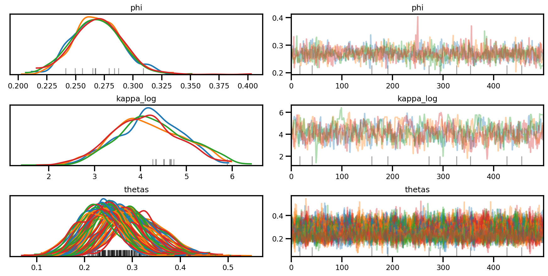
az.plot_trace(az_trace, compact=True);
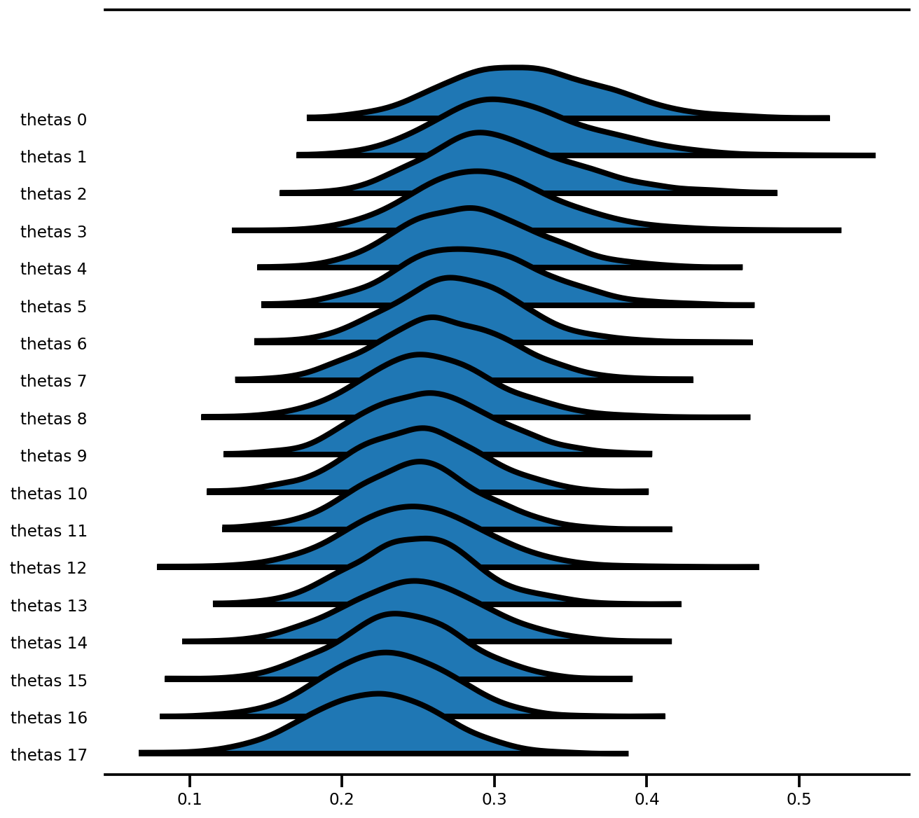
az.plot_forest(az_trace,
               var_names=['thetas'],
               kind='ridgeplot',
               linewidth=4,
               combined=True,
               ridgeplot_overlap=1.5,
               figsize=(9, 8));
혼합 효과 모델(라돈)
PyMC3의 문서의 마지막 모델 : 다단계 모델링을위한 베이지안 방법에 뇌관
이전의 일부 변경 사항(소규모 등)
원시 데이터 로드 및 정리
srrs2 = pd.read_csv('https://raw.githubusercontent.com/pymc-devs/pymc3/master/pymc3/examples/data/srrs2.dat')

srrs2.columns = srrs2.columns.map(str.strip)
srrs_mn = srrs2[srrs2.state=='MN'].copy()
srrs_mn['fips'] = srrs_mn.stfips*1000 + srrs_mn.cntyfips

cty = pd.read_csv('https://raw.githubusercontent.com/pymc-devs/pymc3/master/pymc3/examples/data/cty.dat')
cty_mn = cty[cty.st=='MN'].copy()
cty_mn[ 'fips'] = 1000*cty_mn.stfips + cty_mn.ctfips

srrs_mn = srrs_mn.merge(cty_mn[['fips', 'Uppm']], on='fips')
srrs_mn = srrs_mn.drop_duplicates(subset='idnum')
u = np.log(srrs_mn.Uppm)

n = len(srrs_mn)

srrs_mn.county = srrs_mn.county.map(str.strip)
mn_counties = srrs_mn.county.unique()
counties = len(mn_counties)
county_lookup = dict(zip(mn_counties, range(len(mn_counties))))

county = srrs_mn['county_code'] = srrs_mn.county.replace(county_lookup).values
radon = srrs_mn.activity
srrs_mn['log_radon'] = log_radon = np.log(radon + 0.1).values
floor_measure = srrs_mn.floor.values.astype('float')

# Create new variable for mean of floor across counties
xbar = srrs_mn.groupby('county')['floor'].mean().rename(county_lookup).values
복잡한 변환이 있는 모델의 경우 기능적 스타일로 구현하면 작성 및 테스트가 훨씬 쉬워집니다. 또한 입력된 데이터의 (미니 배치)를 조건으로 하는 log_prob 함수를 프로그래밍 방식으로 훨씬 쉽게 생성할 수 있습니다.
def affine(u_val, x_county, county, floor, gamma, eps, b):
  """Linear equation of the coefficients and the covariates, with broadcasting."""
  return (tf.transpose((gamma[..., 0]
                      + gamma[..., 1]*u_val[:, None]
                      + gamma[..., 2]*x_county[:, None]))
          + tf.gather(eps, county, axis=-1)
          + b*floor)


def gen_radon_model(u_val, x_county, county, floor,
                    mu0=tf.zeros([], dtype, name='mu0')):
  """Creates a joint distribution representing our generative process."""
  return tfd.JointDistributionSequential([
      # sigma_a
      tfd.HalfCauchy(loc=mu0, scale=5.),
      # eps
      lambda sigma_a: tfd.Sample(
          tfd.Normal(loc=mu0, scale=sigma_a), sample_shape=counties),
      # gamma
      tfd.Sample(tfd.Normal(loc=mu0, scale=100.), sample_shape=3),
      # b
      tfd.Sample(tfd.Normal(loc=mu0, scale=100.), sample_shape=1),
      # sigma_y
      tfd.Sample(tfd.HalfCauchy(loc=mu0, scale=5.), sample_shape=1),
      # likelihood
      lambda sigma_y, b, gamma, eps: tfd.Independent(
          tfd.Normal(
              loc=affine(u_val, x_county, county, floor, gamma, eps, b),
              scale=sigma_y
          ),
          reinterpreted_batch_ndims=1
      ),
  ])

contextual_effect2 = gen_radon_model(
    u.values,  xbar[county], county, floor_measure)

@tf.function(autograph=False)
def unnormalized_posterior_log_prob(sigma_a, gamma, eps, b, sigma_y):
  """Computes `joint_log_prob` pinned at `log_radon`."""
  return contextual_effect2.log_prob(
      [sigma_a, gamma, eps, b, sigma_y, log_radon])

assert [4] == unnormalized_posterior_log_prob(
    *contextual_effect2.sample(4)[:-1]).shape
samples = contextual_effect2.sample(4)
pprint([s.shape for s in samples])
[TensorShape([4]),
 TensorShape([4, 85]),
 TensorShape([4, 3]),
 TensorShape([4, 1]),
 TensorShape([4, 1]),
 TensorShape([4, 919])]
contextual_effect2.log_prob_parts(list(samples)[:-1] + [log_radon])
[<tf.Tensor: shape=(4,), dtype=float64, numpy=array([-3.95681828, -2.45693443, -2.53310078, -4.7717536 ])>,
 <tf.Tensor: shape=(4,), dtype=float64, numpy=array([-340.65975204, -217.11139018, -246.50498667, -369.79687704])>,
 <tf.Tensor: shape=(4,), dtype=float64, numpy=array([-20.49822449, -20.38052557, -18.63843525, -17.83096972])>,
 <tf.Tensor: shape=(4,), dtype=float64, numpy=array([-5.94765605, -5.91460848, -6.66169402, -5.53894593])>,
 <tf.Tensor: shape=(4,), dtype=float64, numpy=array([-2.10293999, -4.34186631, -2.10744955, -3.016717  ])>,
 <tf.Tensor: shape=(4,), dtype=float64, numpy=
 array([-29022322.1413861 ,   -114422.36893361,  -8708500.81752865,
           -35061.92497235])>]
변이 추론
의 강력한 기능 중 하나 JointDistribution* 당신이 VI를 위해 쉽게 근사치를 생성 할 수 있다는 것입니다. 예를 들어, meanfield ADVI를 수행하려면 그래프를 검사하고 관찰되지 않은 모든 분포를 정규 분포로 바꾸면 됩니다.
평균 필드 ADVI
당신은 또한에 experimential 기능을 사용할 수 있습니다 tensorflow_probability / 파이썬 / 실험 / VI 기본적으로 아래에 사용 된 것과 같은 논리입니다 변분 근사를 구축하기 위해 (즉, 빌드 근사치에 JointDistribution 사용) 대신하지만, 원래의 공간에서 근사 출력 무한한 공간.
from tensorflow_probability.python.mcmc.transformed_kernel import (
    make_transform_fn, make_transformed_log_prob)
# Wrap logp so that all parameters are in the Real domain
# copied and edited from tensorflow_probability/python/mcmc/transformed_kernel.py
unconstraining_bijectors = [
    tfb.Exp(),
    tfb.Identity(),
    tfb.Identity(),
    tfb.Identity(),
    tfb.Exp()
]

unnormalized_log_prob = lambda *x: contextual_effect2.log_prob(x + (log_radon,))

contextual_effect_posterior = make_transformed_log_prob(
    unnormalized_log_prob,
    unconstraining_bijectors,
    direction='forward',
    # TODO(b/72831017): Disable caching until gradient linkage
    # generally works.
    enable_bijector_caching=False)
# debug
if True:
  # Check the two versions of log_prob - they should be different given the Jacobian
  rv_samples = contextual_effect2.sample(4)

  _inverse_transform = make_transform_fn(unconstraining_bijectors, 'inverse')
  _forward_transform = make_transform_fn(unconstraining_bijectors, 'forward')

  pprint([
      unnormalized_log_prob(*rv_samples[:-1]),
      contextual_effect_posterior(*_inverse_transform(rv_samples[:-1])),
      unnormalized_log_prob(
          *_forward_transform(
              tf.zeros_like(a, dtype=dtype) for a in rv_samples[:-1])
      ),
      contextual_effect_posterior(
          *[tf.zeros_like(a, dtype=dtype) for a in rv_samples[:-1]]
      ),
  ])
[<tf.Tensor: shape=(4,), dtype=float64, numpy=array([-1.73354969e+04, -5.51622488e+04, -2.77754609e+08, -1.09065161e+07])>,
 <tf.Tensor: shape=(4,), dtype=float64, numpy=array([-1.73331358e+04, -5.51582029e+04, -2.77754602e+08, -1.09065134e+07])>,
 <tf.Tensor: shape=(4,), dtype=float64, numpy=array([-1992.10420767, -1992.10420767, -1992.10420767, -1992.10420767])>,
 <tf.Tensor: shape=(4,), dtype=float64, numpy=array([-1992.10420767, -1992.10420767, -1992.10420767, -1992.10420767])>]
# Build meanfield ADVI for a jointdistribution
# Inspect the input jointdistribution and replace the list of distribution with
# a list of Normal distribution, each with the same shape.
def build_meanfield_advi(jd_list, observed_node=-1):
  """
  The inputted jointdistribution needs to be a batch version
  """
  # Sample to get a list of Tensors
  list_of_values = jd_list.sample(1)  # <== sample([]) might not work

  # Remove the observed node
  list_of_values.pop(observed_node)

  # Iterate the list of Tensor to a build a list of Normal distribution (i.e.,
  # the Variational posterior)
  distlist = []
  for i, value in enumerate(list_of_values):
    dtype = value.dtype
    rv_shape = value[0].shape
    loc = tf.Variable(
        tf.random.normal(rv_shape, dtype=dtype),
        name='meanfield_%s_mu' % i,
        dtype=dtype)
    scale = tfp.util.TransformedVariable(
        tf.fill(rv_shape, value=tf.constant(0.02, dtype)),
        tfb.Softplus(),
        name='meanfield_%s_scale' % i,
    )

    approx_node = tfd.Normal(loc=loc, scale=scale)
    if loc.shape == ():
      distlist.append(approx_node)
    else:
      distlist.append(
          # TODO: make the reinterpreted_batch_ndims more flexible (for
          # minibatch etc)
          tfd.Independent(approx_node, reinterpreted_batch_ndims=1)
      )

  # pass list to JointDistribution to initiate the meanfield advi
  meanfield_advi = tfd.JointDistributionSequential(distlist)
  return meanfield_advi
advi = build_meanfield_advi(contextual_effect2, observed_node=-1)

# Check the logp and logq
advi_samples = advi.sample(4)
pprint([
  advi.log_prob(advi_samples),
  contextual_effect_posterior(*advi_samples)
  ])
[<tf.Tensor: shape=(4,), dtype=float64, numpy=array([231.26836839, 229.40755095, 227.10287879, 224.05914594])>,
 <tf.Tensor: shape=(4,), dtype=float64, numpy=array([-10615.93542431, -11743.21420129, -10376.26732337, -11338.00600103])>]
opt = tf.optimizers.Adam(learning_rate=.1)
@tf.function(experimental_compile=True)
def run_approximation():
loss_ = tfp.vi.fit_surrogate_posterior(
contextual_effect_posterior,
surrogate_posterior=advi,
optimizer=opt,
sample_size=10,
num_steps=300)
return loss_
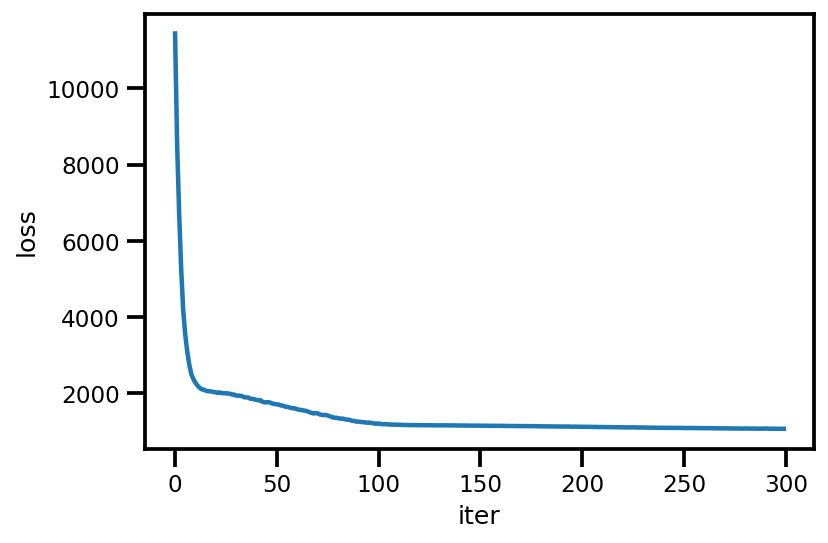
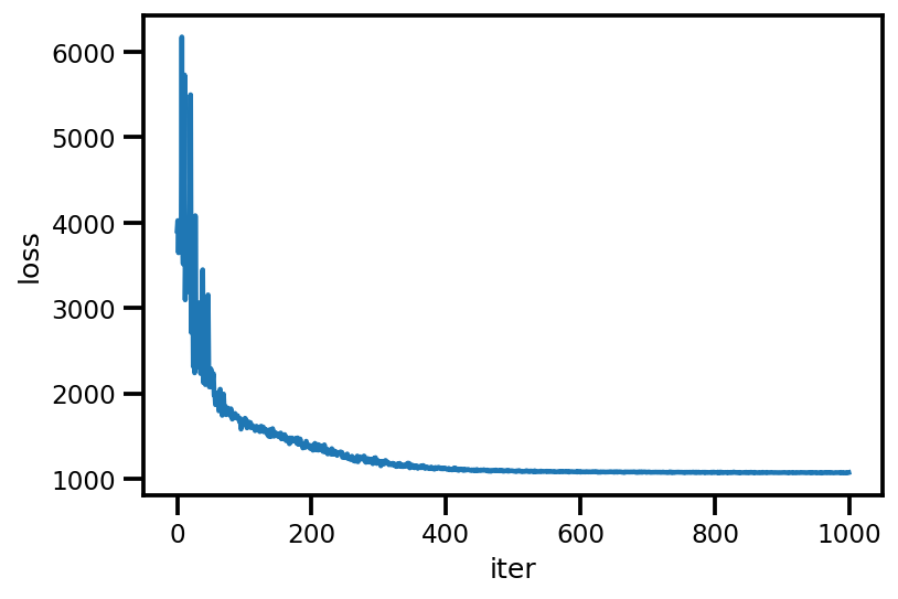
loss_ = run_approximation()
plt.plot(loss_);
plt.xlabel('iter');
plt.ylabel('loss');
graph_info = contextual_effect2.resolve_graph()
approx_param = dict()
free_param = advi.trainable_variables
for i, (rvname, param) in enumerate(graph_info[:-1]):
  approx_param[rvname] = {"mu": free_param[i*2].numpy(),
                          "sd": free_param[i*2+1].numpy()}
approx_param.keys()
dict_keys(['sigma_a', 'eps', 'gamma', 'b', 'sigma_y'])
approx_param['gamma']
{'mu': array([1.28145814, 0.70365287, 1.02689857]),
 'sd': array([-3.6604972 , -2.68153218, -2.04176524])}
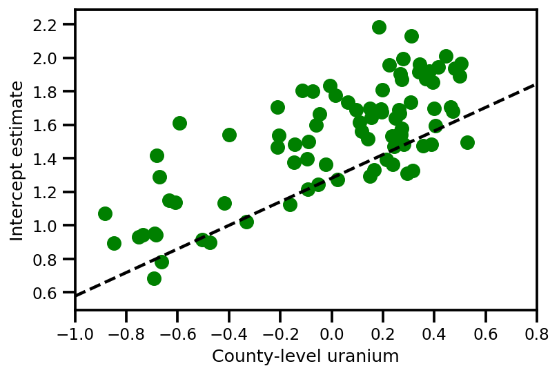
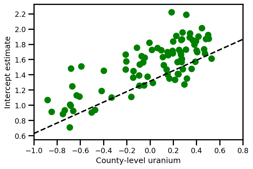
a_means = (approx_param['gamma']['mu'][0]
         + approx_param['gamma']['mu'][1]*u.values
         + approx_param['gamma']['mu'][2]*xbar[county]
         + approx_param['eps']['mu'][county])
_, index = np.unique(county, return_index=True)
plt.scatter(u.values[index], a_means[index], color='g')

xvals = np.linspace(-1, 0.8)
plt.plot(xvals,
         approx_param['gamma']['mu'][0]+approx_param['gamma']['mu'][1]*xvals,
         'k--')
plt.xlim(-1, 0.8)

plt.xlabel('County-level uranium');
plt.ylabel('Intercept estimate');
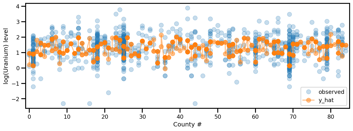
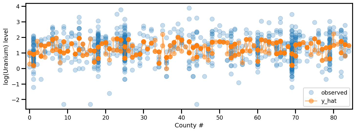
y_est = (approx_param['gamma']['mu'][0]
        + approx_param['gamma']['mu'][1]*u.values
        + approx_param['gamma']['mu'][2]*xbar[county]
        + approx_param['eps']['mu'][county]
        + approx_param['b']['mu']*floor_measure)

_, ax = plt.subplots(1, 1, figsize=(12, 4))
ax.plot(county, log_radon, 'o', alpha=.25, label='observed')
ax.plot(county, y_est, '-o', lw=2, alpha=.5, label='y_hat')
ax.set_xlim(-1, county.max()+1)
plt.legend(loc='lower right')
ax.set_xlabel('County #')
ax.set_ylabel('log(Uranium) level');
전체 순위 ADVI
전체 순위 ADVI의 경우, 우리는 다변수 가우시안을 사용하여 사후값을 근사화하려고 합니다.
USE_FULLRANK = True
*prior_tensors, _ = contextual_effect2.sample()

mapper = Mapper(prior_tensors,
                [tfb.Identity() for _ in prior_tensors],
                contextual_effect2.event_shape[:-1])
rv_shape = ps.shape(mapper.flatten_and_concat(mapper.list_of_tensors))
init_val = tf.random.normal(rv_shape, dtype=dtype)
loc = tf.Variable(init_val, name='loc', dtype=dtype)

if USE_FULLRANK:
  # cov_param = tfp.util.TransformedVariable(
  #     10. * tf.eye(rv_shape[0], dtype=dtype),
  #     tfb.FillScaleTriL(),
  #     name='cov_param'
  #     )
  FillScaleTriL = tfb.FillScaleTriL(
        diag_bijector=tfb.Chain([
          tfb.Shift(tf.cast(.01, dtype)),
          tfb.Softplus(),
          tfb.Shift(tf.cast(np.log(np.expm1(1.)), dtype))]),
        diag_shift=None)
  cov_param = tfp.util.TransformedVariable(
      .02 * tf.eye(rv_shape[0], dtype=dtype),
      FillScaleTriL,
      name='cov_param')
  advi_approx = tfd.MultivariateNormalTriL(
      loc=loc, scale_tril=cov_param)
else:
  # An alternative way to build meanfield ADVI.
  cov_param = tfp.util.TransformedVariable(
      .02 * tf.ones(rv_shape, dtype=dtype),
      tfb.Softplus(),
      name='cov_param'
      )
  advi_approx = tfd.MultivariateNormalDiag(
      loc=loc, scale_diag=cov_param)

contextual_effect_posterior2 = lambda x: contextual_effect_posterior(
    *mapper.split_and_reshape(x)
)

# Check the logp and logq
advi_samples = advi_approx.sample(7)
pprint([
  advi_approx.log_prob(advi_samples),
  contextual_effect_posterior2(advi_samples)
  ])
[<tf.Tensor: shape=(7,), dtype=float64, numpy=
array([238.81841799, 217.71022639, 234.57207103, 230.0643819 ,
       243.73140943, 226.80149702, 232.85184209])>,
 <tf.Tensor: shape=(7,), dtype=float64, numpy=
array([-3638.93663169, -3664.25879314, -3577.69371677, -3696.25705312,
       -3689.12130489, -3777.53698383, -3659.4982734 ])>]
learning_rate = tf.optimizers.schedules.ExponentialDecay(
    initial_learning_rate=1e-2,
    decay_steps=10,
    decay_rate=0.99,
    staircase=True)

opt = tf.optimizers.Adam(learning_rate=learning_rate)

@tf.function(experimental_compile=True)
def run_approximation():
  loss_ = tfp.vi.fit_surrogate_posterior(
        contextual_effect_posterior2,
        surrogate_posterior=advi_approx,
        optimizer=opt,
        sample_size=10,
        num_steps=1000)
  return loss_

loss_ = run_approximation()
plt.plot(loss_);
plt.xlabel('iter');
plt.ylabel('loss');
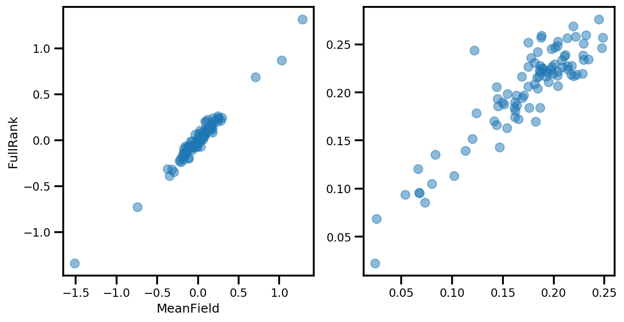
# debug
if True:
  _, ax = plt.subplots(1, 2, figsize=(10, 5))
  ax[0].plot(mapper.flatten_and_concat(advi.mean()), advi_approx.mean(), 'o', alpha=.5)
  ax[1].plot(mapper.flatten_and_concat(advi.stddev()), advi_approx.stddev(), 'o', alpha=.5)
  ax[0].set_xlabel('MeanField')
  ax[0].set_ylabel('FullRank')
graph_info = contextual_effect2.resolve_graph()
approx_param = dict()

free_param_mean = mapper.split_and_reshape(advi_approx.mean())
free_param_std = mapper.split_and_reshape(advi_approx.stddev())
for i, (rvname, param) in enumerate(graph_info[:-1]):
  approx_param[rvname] = {"mu": free_param_mean[i].numpy(),
                          "cov_info": free_param_std[i].numpy()}
a_means = (approx_param['gamma']['mu'][0]
         + approx_param['gamma']['mu'][1]*u.values
         + approx_param['gamma']['mu'][2]*xbar[county]
         + approx_param['eps']['mu'][county])
_, index = np.unique(county, return_index=True)
plt.scatter(u.values[index], a_means[index], color='g')

xvals = np.linspace(-1, 0.8)
plt.plot(xvals,
         approx_param['gamma']['mu'][0]+approx_param['gamma']['mu'][1]*xvals,
         'k--')
plt.xlim(-1, 0.8)

plt.xlabel('County-level uranium');
plt.ylabel('Intercept estimate');
y_est = (approx_param['gamma']['mu'][0]
         + approx_param['gamma']['mu'][1]*u.values
         + approx_param['gamma']['mu'][2]*xbar[county]
         + approx_param['eps']['mu'][county]
         + approx_param['b']['mu']*floor_measure)

_, ax = plt.subplots(1, 1, figsize=(12, 4))
ax.plot(county, log_radon, 'o', alpha=.25, label='observed')
ax.plot(county, y_est, '-o', lw=2, alpha=.5, label='y_hat')
ax.set_xlim(-1, county.max()+1)
plt.legend(loc='lower right')
ax.set_xlabel('County #')
ax.set_ylabel('log(Uranium) level');
베타-베르누이 혼합물 모델
여러 검토자가 일부 항목에 레이블을 지정하고 알 수 없는(진정한) 잠재 레이블을 지정하는 혼합 모델입니다.
dtype = tf.float32
n = 50000    # number of examples reviewed
p_bad_ = 0.1 # fraction of bad events
m = 5        # number of reviewers for each example
rcl_ = .35 + np.random.rand(m)/10
prc_ = .65 + np.random.rand(m)/10

# PARAMETER TRANSFORMATION
tpr = rcl_
fpr = p_bad_*tpr*(1./prc_-1.)/(1.-p_bad_)
tnr = 1 - fpr

# broadcast to m reviewer.
batch_prob = np.asarray([tpr, fpr]).T
mixture = tfd.Mixture(
    tfd.Categorical(
        probs=[p_bad_, 1-p_bad_]),
    [
        tfd.Independent(tfd.Bernoulli(probs=tpr), 1),
        tfd.Independent(tfd.Bernoulli(probs=fpr), 1),
    ])
# Generate reviewer response
X_tf = mixture.sample([n])

# run once to always use the same array as input
# so we can compare the estimation from different
# inference method.
X_np = X_tf.numpy()
# batched Mixture model
mdl_mixture = tfd.JointDistributionSequential([
    tfd.Sample(tfd.Beta(5., 2.), m),
    tfd.Sample(tfd.Beta(2., 2.), m),
    tfd.Sample(tfd.Beta(1., 10), 1),
    lambda p_bad, rcl, prc: tfd.Sample(
        tfd.Mixture(
            tfd.Categorical(
                probs=tf.concat([p_bad, 1.-p_bad], -1)),
            [
              tfd.Independent(tfd.Bernoulli(
                  probs=rcl), 1),
              tfd.Independent(tfd.Bernoulli(
                  probs=p_bad*rcl*(1./prc-1.)/(1.-p_bad)), 1)
             ]
      ), (n, )),
    ])

mdl_mixture.resolve_graph()
(('prc', ()), ('rcl', ()), ('p_bad', ()), ('x', ('p_bad', 'rcl', 'prc')))
prc, rcl, p_bad, x = mdl_mixture.sample(4)
x.shape
TensorShape([4, 50000, 5])
mdl_mixture.log_prob_parts([prc, rcl, p_bad, X_np[np.newaxis, ...]])
[<tf.Tensor: shape=(4,), dtype=float32, numpy=array([1.4828572, 2.957961 , 2.9355168, 2.6116824], dtype=float32)>,
 <tf.Tensor: shape=(4,), dtype=float32, numpy=array([-0.14646745,  1.3308513 ,  1.1205603 ,  0.5441705 ], dtype=float32)>,
 <tf.Tensor: shape=(4,), dtype=float32, numpy=array([1.3733709, 1.8020535, 2.1865845, 1.5701319], dtype=float32)>,
 <tf.Tensor: shape=(4,), dtype=float32, numpy=array([-54326.664, -52683.93 , -64407.67 , -55007.895], dtype=float32)>]
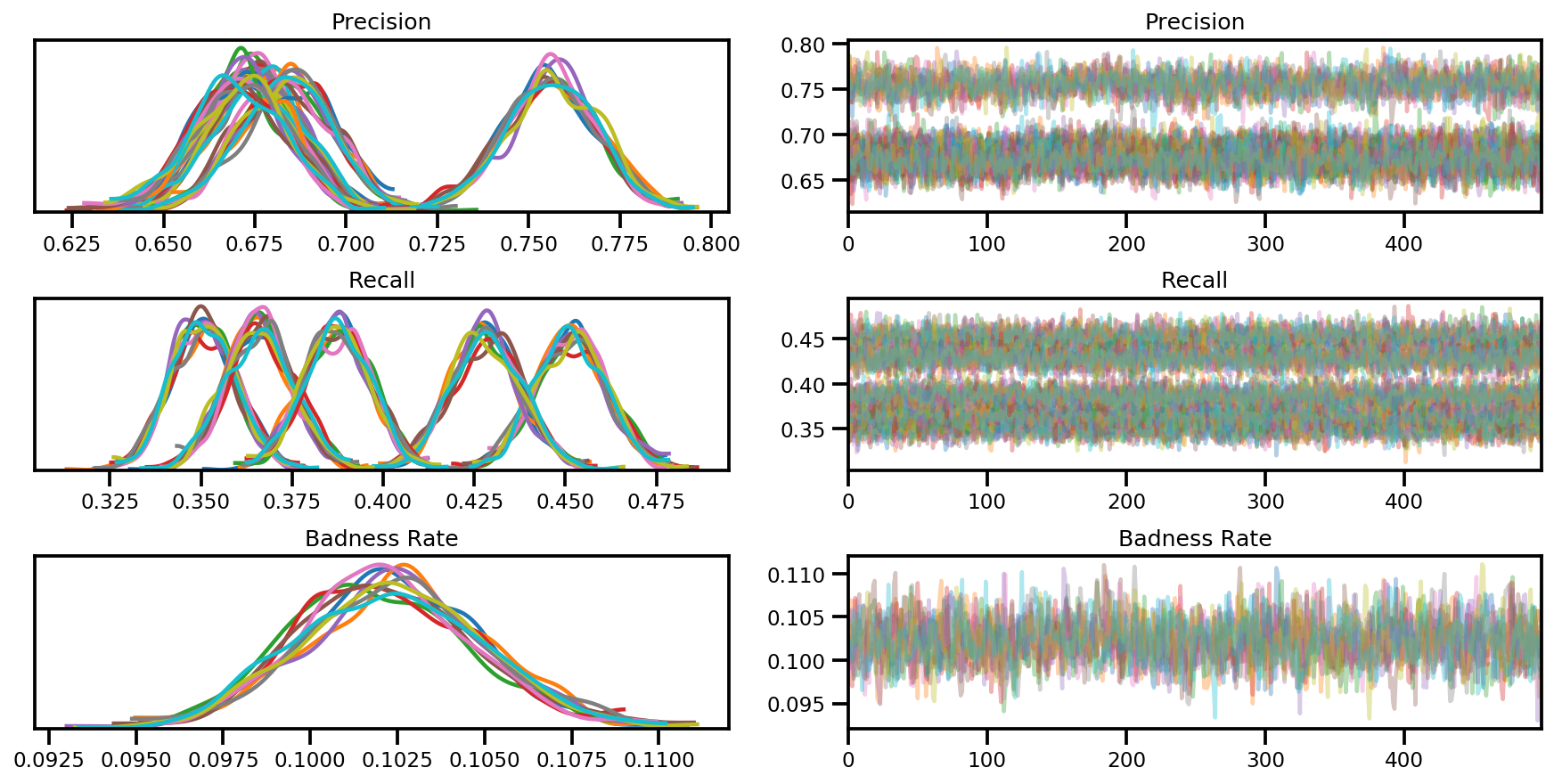
추론(NUTS)
nchain = 10
prc, rcl, p_bad, _ = mdl_mixture.sample(nchain)
initial_chain_state = [prc, rcl, p_bad]

# Since MCMC operates over unconstrained space, we need to transform the
# samples so they live in real-space.
unconstraining_bijectors = [
    tfb.Sigmoid(),       # Maps R to [0, 1].
    tfb.Sigmoid(),       # Maps R to [0, 1].
    tfb.Sigmoid(),       # Maps R to [0, 1].
]
step_size = [tf.cast(i, dtype=dtype) for i in [1e-3, 1e-3, 1e-3]]

X_expanded = X_np[np.newaxis, ...]
target_log_prob_fn = lambda *x: mdl_mixture.log_prob(x + (X_expanded, ))

samples, sampler_stat = run_chain(
    initial_chain_state, step_size, target_log_prob_fn,
    unconstraining_bijectors, burnin=100)
# using the pymc3 naming convention
sample_stats_name = ['lp', 'tree_size', 'diverging', 'energy', 'mean_tree_accept']
sample_stats = {k:v.numpy().T for k, v in zip(sample_stats_name, sampler_stat)}
sample_stats['tree_size'] = np.diff(sample_stats['tree_size'], axis=1)

var_name = ['Precision', 'Recall', 'Badness Rate']
posterior = {k:np.swapaxes(v.numpy(), 1, 0)
             for k, v in zip(var_name, samples)}

az_trace = az.from_dict(posterior=posterior, sample_stats=sample_stats)
axes = az.plot_trace(az_trace, compact=True);