
베이지안 모델 선택
| | |  GitHub에서 소스 보기 GitHub에서 소스 보기 | |
수입품
import numpy as np
import tensorflow.compat.v2 as tf
tf.enable_v2_behavior()
import tensorflow_probability as tfp
from tensorflow_probability import distributions as tfd

from matplotlib import pylab as plt
%matplotlib inline
import scipy.stats
작업: 여러 변경점으로 변경점 감지
변경점 감지 작업을 고려하십시오. 이벤트는 데이터를 생성하는 일부 시스템 또는 프로세스의 (관측되지 않은) 상태의 갑작스러운 변화에 의해 구동되는 시간이 지남에 따라 변하는 속도로 발생합니다.
예를 들어 다음과 같은 일련의 카운트를 관찰할 수 있습니다.
true_rates = [40, 3, 20, 50]
true_durations = [10, 20, 5, 35]

observed_counts = tf.concat(
    [tfd.Poisson(rate).sample(num_steps)
     for (rate, num_steps) in zip(true_rates, true_durations)], axis=0)

plt.plot(observed_counts)
[<matplotlib.lines.Line2D at 0x7f7589bdae10>]
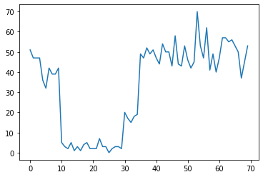
이는 데이터 센터의 오류 수, 웹 페이지 방문자 수, 네트워크 링크의 패킷 수 등을 나타낼 수 있습니다.
데이터를 보는 것만으로는 얼마나 많은 별개의 시스템 체제가 있는지 완전히 명확하지 않다는 점에 유의하십시오. 세 개의 전환점이 각각 어디에서 발생하는지 알 수 있습니까?
알려진 상태 수
우리는 먼저 관찰되지 않은 상태의 수가 선험적으로 알려진 (아마도 비현실적인) 경우를 고려할 것입니다. 여기에서 우리는 4개의 잠재 상태가 있다는 것을 알고 있다고 가정합니다.
우리는 스위칭 (불균일) 포아송 프로세스로이 문제를 모델 : 각 시점에서 발생하는 이벤트의 수는 포아송 분포 및 이벤트의 레이트가 관측 시스템 상태에 의해 결정된다 \(z_t\):
\[x_t \sim \text{Poisson}(\lambda_{z_t})\]
잠재 상태 이산 : \(z_t \in \{1, 2, 3, 4\}\), 그래서 \(\lambda = [\lambda_1, \lambda_2, \lambda_3, \lambda_4]\) 각각의 상태에 대한 푸 아송 레이트를 함유하는 단순한 벡터이다. 시간이 지남에 따라 국가의 발전을 모델링하기 위해, 우리는 간단한 전환 모델을 정의 할 것이다 \(p(z_t | z_{t-1})\):의 각 단계에서 우리는 약간의 확률로 이전의 상태로 유지 가정 해 봅시다 \(p\), 확률과 \(1-p\) A와 우리의 전환 무작위로 균일하게 다른 상태. 초기 상태도 무작위로 균일하게 선택되므로 다음을 얻습니다.
\[ \begin{align*} z_1 &\sim \text{Categorical}\left(\left\{\frac{1}{4}, \frac{1}{4}, \frac{1}{4}, \frac{1}{4}\right\}\right)\\ z_t | z_{t-1} &\sim \text{Categorical}\left(\left\{\begin{array}{cc}p & \text{if } z_t = z_{t-1} \\ \frac{1-p}{4-1} & \text{otherwise}\end{array}\right\}\right) \end{align*}\]
이러한 가정은 해당 숨겨진 마르코프 모델 포아송 배출량. 우리는 사용 TFP에서 그들을 인코딩 할 수 tfd.HiddenMarkovModel . 먼저, 초기 상태에 대한 천이 행렬과 유니폼 사전을 정의합니다.
num_states = 4
initial_state_logits = tf.zeros([num_states]) # uniform distribution

daily_change_prob = 0.05
transition_probs = tf.fill([num_states, num_states],
                           daily_change_prob / (num_states - 1))
transition_probs = tf.linalg.set_diag(transition_probs,
                                      tf.fill([num_states],
                                              1 - daily_change_prob))

print("Initial state logits:\n{}".format(initial_state_logits))
print("Transition matrix:\n{}".format(transition_probs))
Initial state logits:
[0. 0. 0. 0.]
Transition matrix:
[[0.95       0.01666667 0.01666667 0.01666667]
 [0.01666667 0.95       0.01666667 0.01666667]
 [0.01666667 0.01666667 0.95       0.01666667]
 [0.01666667 0.01666667 0.01666667 0.95      ]]
다음으로, 우리는 구축 tfd.HiddenMarkovModel 각 시스템의 상태와 관련된 요금을 표현하기 위해 학습 가능한 변수를 사용하여 배포. 양수 값이 되도록 로그 공간의 비율을 매개변수화합니다.
# Define variable to represent the unknown log rates.
trainable_log_rates = tf.Variable(
  tf.math.log(tf.reduce_mean(observed_counts)) +
  tf.random.stateless_normal([num_states], seed=(42, 42)),
  name='log_rates')

hmm = tfd.HiddenMarkovModel(
  initial_distribution=tfd.Categorical(
      logits=initial_state_logits),
  transition_distribution=tfd.Categorical(probs=transition_probs),
  observation_distribution=tfd.Poisson(log_rate=trainable_log_rates),
  num_steps=len(observed_counts))
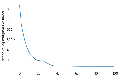
마지막으로, 우리는 환율 전에 약하게 정보를 로그 정규 포함한 모델의 전체 로그 밀도를 정의하고 계산하는 최적화를 실행 최대에게 사후 관찰 카운트 데이터 (MAP) 적합합니다.
rate_prior = tfd.LogNormal(5, 5)

def log_prob():
 return (tf.reduce_sum(rate_prior.log_prob(tf.math.exp(trainable_log_rates))) +
         hmm.log_prob(observed_counts))

losses = tfp.math.minimize(
    lambda: -log_prob(),
    optimizer=tf.optimizers.Adam(learning_rate=0.1),
    num_steps=100)
plt.plot(losses)
plt.ylabel('Negative log marginal likelihood')
Text(0, 0.5, 'Negative log marginal likelihood')
rates = tf.exp(trainable_log_rates)
print("Inferred rates: {}".format(rates))
print("True rates: {}".format(true_rates))
Inferred rates: [ 2.8302798 49.58499   41.928307  17.35112  ]
True rates: [40, 3, 20, 50]
효과가 있었다! 이 모델의 잠재 상태는 순열까지만 식별할 수 있으므로 우리가 복구한 비율은 다른 순서로 되어 있고 약간의 노이즈가 있지만 일반적으로 꽤 잘 일치합니다.
상태 궤적 회복
이제 우리는 모델에 맞게 했으므로 우리는 모델이 시스템은 각 시간 단계에서 있었다 믿는 상태를 재구성 할 수 있습니다.
이것은 후방 추론 작업입니다 : 관찰 카운트 주어진 \(x_{1:T}\) 및 모델 매개 변수 (요금) \(\lambda\), 우리는 사후 분포에 따라 개별 잠재 변수의 순서를 추론 할 \(p(z_{1:T} | x_{1:T}, \lambda)\). 은닉 마르코프 모델에서 표준 메시지 전달 알고리즘을 사용하여 이 분포의 한계 및 기타 속성을 효율적으로 계산할 수 있습니다. 특히, posterior_marginals 있어서 효율적으로합니다 (하여 계산한다 전후 알고리즘 한계 확률 분포) \(p(Z_t = z_t | x_{1:T})\) 이산 잠복 상태 위에 \(Z_t\) 각 시간 단계에서의 \(t\).
# Runs forward-backward algorithm to compute marginal posteriors.
posterior_dists = hmm.posterior_marginals(observed_counts)
posterior_probs = posterior_dists.probs_parameter().numpy()
사후 확률을 플로팅하여 데이터에 대한 모델의 "설명"을 복구합니다. 어느 시점에서 각 상태가 활성화됩니까?
def plot_state_posterior(ax, state_posterior_probs, title):
  ln1 = ax.plot(state_posterior_probs, c='blue', lw=3, label='p(state | counts)')
  ax.set_ylim(0., 1.1)
  ax.set_ylabel('posterior probability')
  ax2 = ax.twinx()
  ln2 = ax2.plot(observed_counts, c='black', alpha=0.3, label='observed counts')
  ax2.set_title(title)
  ax2.set_xlabel("time")
  lns = ln1+ln2
  labs = [l.get_label() for l in lns]
  ax.legend(lns, labs, loc=4)
  ax.grid(True, color='white')
  ax2.grid(False)

fig = plt.figure(figsize=(10, 10))
plot_state_posterior(fig.add_subplot(2, 2, 1),
                     posterior_probs[:, 0],
                     title="state 0 (rate {:.2f})".format(rates[0]))
plot_state_posterior(fig.add_subplot(2, 2, 2),
                     posterior_probs[:, 1],
                     title="state 1 (rate {:.2f})".format(rates[1]))
plot_state_posterior(fig.add_subplot(2, 2, 3),
                     posterior_probs[:, 2],
                     title="state 2 (rate {:.2f})".format(rates[2]))
plot_state_posterior(fig.add_subplot(2, 2, 4),
                     posterior_probs[:, 3],
                     title="state 3 (rate {:.2f})".format(rates[3]))
plt.tight_layout()
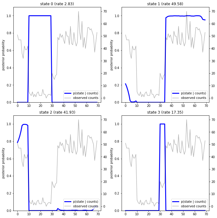
이 (단순한) 경우에 우리는 모델이 일반적으로 매우 확신한다는 것을 알 수 있습니다. 대부분의 시간 단계에서 기본적으로 모든 확률 질량을 네 가지 상태 중 하나에 할당합니다. 다행히 설명이 합리적으로 보입니다!
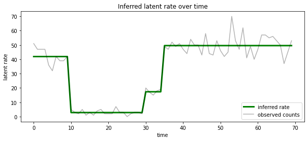
우리는 또한 하나의 설명에 확률 적 후방을 응축, 각 시간 단계에서 가장 가능성이 잠재 상태와 관련된 속도의 관점에서이 후방을 시각화 할 수 있습니다 :
most_probable_states = hmm.posterior_mode(observed_counts)
most_probable_rates = tf.gather(rates, most_probable_states)
fig = plt.figure(figsize=(10, 4))
ax = fig.add_subplot(1, 1, 1)
ax.plot(most_probable_rates, c='green', lw=3, label='inferred rate')
ax.plot(observed_counts, c='black', alpha=0.3, label='observed counts')
ax.set_ylabel("latent rate")
ax.set_xlabel("time")
ax.set_title("Inferred latent rate over time")
ax.legend(loc=4)
<matplotlib.legend.Legend at 0x7f75849e70f0>
알 수 없는 상태 수
실제 문제에서는 우리가 모델링하는 시스템의 '실제' 상태 수를 모를 수 있습니다. 이것이 항상 문제가 되는 것은 아닙니다. 알려지지 않은 상태의 ID에 대해 특별히 신경 쓰지 않는다면, 모델에 필요한 것보다 더 많은 상태로 모델을 실행하고 많은 복제본을 학습할 수 있습니다. 실제 상태의 사본. 그러나 잠재 상태의 '실제' 수를 추론하는 데 관심이 있다고 가정해 보겠습니다.
우리의 경우로 이것을 볼 수 있습니다 베이지안 모델 선택 : 우리는 후보 모델의 집합, 잠재 상태의 다른 번호와 함께 있고, 우리는 가장 가능성이 관측 된 데이터를 생성 한 위해 하나를 선택합니다. 이를 위해, 우리는 우리가 또한 모델 자체에 사전을 추가 할 수 있습니다 (각 모델에서 데이터의 한계 가능성을 계산하지만이 분석에 필요하지 않습니다하며 베이지안 오캄의 면도날은 인코딩 A와 충분한 것으로 판명 더 단순한 모델에 대한 선호).
불행하게도, 둘 이상의 통합하고 분리 된 상태의 진정한 한계 가능성, \(z_{1:T}\) 과 (벡터) 속도 매개 변수 \(\lambda\), \(p(x_{1:T}) = \int p(x_{1:T}, z_{1:T}, \lambda) dz d\lambda,\) 이 모델 다루기 쉬운 없습니다. 편의를 위해, 우리는 소위 "사용하여 대략 것 경험적 베이 즈를 "또는 추정 "II 최대 가능성을 입력합니다"대신에 완전히 (알 수없는) 속도 매개 변수를 통합 \(\lambda\) 각 시스템의 상태와 관련된, 우리가 최적화거야 그들의 가치에 대해:
\[\tilde{p}(x_{1:T}) = \max_\lambda \int p(x_{1:T}, z_{1:T}, \lambda) dz\]
이 근사는 과적합될 수 있습니다. 즉, 실제 한계 가능성보다 더 복잡한 모델을 선호합니다. 우리는이 하한 변분 최적화, 또는 몬테카를로 추정과 같은 사용하여, 예를 들면 충실 근사치를 고려할 수 어닐링 중요성 샘플링을 ; 이것들은 (슬프게도) 이 노트북의 범위를 벗어납니다. (베이지안 모델 선택 및 근사, 우수한 제 7 장에 대한 자세한 내용은 기계 학습 : 확률 적 관점은 좋은 참조입니다.)
원칙적으로, 우리는 단순히 서로 다른 값으로 여러 번 위의 최적화를 다시 실행하여이 모델 비교를 할 수 num_states ,하지만 많은 작업이 될 것입니다. 여기에서 우리는 TFP의 사용, 병렬로 여러 모델을 고려하는 방법을 보여 드리겠습니다 batch_shape 벡터화를위한 메커니즘을.
전환 매트릭스 및 초기 상태에 앞서 : 오히려 단일 모델 설명을 구축하는 것보다, 지금 우리가 전이 행렬 이전 logits, 각 후보 모델까지 하나의 배치 세우겠다 max_num_states . 쉬운 일괄 처리를 위해 모든 계산이 동일한 '모양'을 갖도록 해야 합니다. 이것은 우리가 맞출 가장 큰 모델의 치수와 일치해야 합니다. 더 작은 모델을 처리하기 위해 상태 공간의 최상위 차원에 해당 설명을 '임베딩'하여 나머지 차원을 사용되지 않는 더미 상태로 효과적으로 처리할 수 있습니다.
max_num_states = 10

def build_latent_state(num_states, max_num_states, daily_change_prob=0.05):

  # Give probability exp(-100) ~= 0 to states outside of the current model.
  active_states_mask = tf.concat([tf.ones([num_states]),
                                  tf.zeros([max_num_states - num_states])],
                                 axis=0)
  initial_state_logits = -100. * (1 - active_states_mask)

  # Build a transition matrix that transitions only within the current
  # `num_states` states.
  transition_probs = tf.fill([num_states, num_states],
                             0. if num_states == 1
                             else daily_change_prob / (num_states - 1))
  padded_transition_probs = tf.eye(max_num_states) + tf.pad(
      tf.linalg.set_diag(transition_probs,
                         tf.fill([num_states], - daily_change_prob)),
      paddings=[(0, max_num_states - num_states),
                (0, max_num_states - num_states)])

  return initial_state_logits, padded_transition_probs

# For each candidate model, build the initial state prior and transition matrix.
batch_initial_state_logits = []
batch_transition_probs = []
for num_states in range(1, max_num_states+1):
  initial_state_logits, transition_probs = build_latent_state(
      num_states=num_states,
      max_num_states=max_num_states)
  batch_initial_state_logits.append(initial_state_logits)
  batch_transition_probs.append(transition_probs)

batch_initial_state_logits = tf.stack(batch_initial_state_logits)
batch_transition_probs = tf.stack(batch_transition_probs)
print("Shape of initial_state_logits: {}".format(batch_initial_state_logits.shape))
print("Shape of transition probs: {}".format(batch_transition_probs.shape))
print("Example initial state logits for num_states==3:\n{}".format(batch_initial_state_logits[2, :]))
print("Example transition_probs for num_states==3:\n{}".format(batch_transition_probs[2, :, :]))
Shape of initial_state_logits: (10, 10)
Shape of transition probs: (10, 10, 10)
Example initial state logits for num_states==3:
[  -0.   -0.   -0. -100. -100. -100. -100. -100. -100. -100.]
Example transition_probs for num_states==3:
[[0.95  0.025 0.025 0.    0.    0.    0.    0.    0.    0.   ]
 [0.025 0.95  0.025 0.    0.    0.    0.    0.    0.    0.   ]
 [0.025 0.025 0.95  0.    0.    0.    0.    0.    0.    0.   ]
 [0.    0.    0.    1.    0.    0.    0.    0.    0.    0.   ]
 [0.    0.    0.    0.    1.    0.    0.    0.    0.    0.   ]
 [0.    0.    0.    0.    0.    1.    0.    0.    0.    0.   ]
 [0.    0.    0.    0.    0.    0.    1.    0.    0.    0.   ]
 [0.    0.    0.    0.    0.    0.    0.    1.    0.    0.   ]
 [0.    0.    0.    0.    0.    0.    0.    0.    1.    0.   ]
 [0.    0.    0.    0.    0.    0.    0.    0.    0.    1.   ]]
이제 위와 같이 진행합니다. 이 시간은 우리에 추가 배치 차원을 사용합니다 trainable_rates 별도로 고려중인 각 모델에 대한 비율에 맞게.
trainable_log_rates = tf.Variable(
    tf.fill([batch_initial_state_logits.shape[0], max_num_states],
            tf.math.log(tf.reduce_mean(observed_counts))) +
     tf.random.stateless_normal([1, max_num_states], seed=(42, 42)),
     name='log_rates')

hmm = tfd.HiddenMarkovModel(
  initial_distribution=tfd.Categorical(
      logits=batch_initial_state_logits),
  transition_distribution=tfd.Categorical(probs=batch_transition_probs),
  observation_distribution=tfd.Poisson(log_rate=trainable_log_rates),
  num_steps=len(observed_counts))
print("Defined HMM with batch shape: {}".format(hmm.batch_shape))
Defined HMM with batch shape: (10,)
총 로그 확률을 계산할 때 각 모델 구성 요소에서 실제로 사용되는 비율에 대한 사전 정보만 합산하도록 주의합니다.
rate_prior = tfd.LogNormal(5, 5)

def log_prob():
  prior_lps = rate_prior.log_prob(tf.math.exp(trainable_log_rates))
  prior_lp = tf.stack(
      [tf.reduce_sum(prior_lps[i, :i+1]) for i in range(max_num_states)])
  return prior_lp + hmm.log_prob(observed_counts)
이제 우리는 동시에 모든 후보 모델을 피팅, 우리가 건설 한 배치 목적을 최적화 :
losses = tfp.math.minimize(
lambda: -log_prob(),
optimizer=tf.optimizers.Adam(0.1),
num_steps=100)
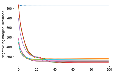
plt.plot(losses)
plt.ylabel('Negative log marginal likelihood')
Text(0, 0.5, 'Negative log marginal likelihood')
num_states = np.arange(1, max_num_states+1)
plt.plot(num_states, -losses[-1])
plt.ylim([-400, -200])
plt.ylabel("marginal likelihood $\\tilde{p}(x)$")
plt.xlabel("number of latent states")
plt.title("Model selection on latent states")
Text(0.5, 1.0, 'Model selection on latent states')
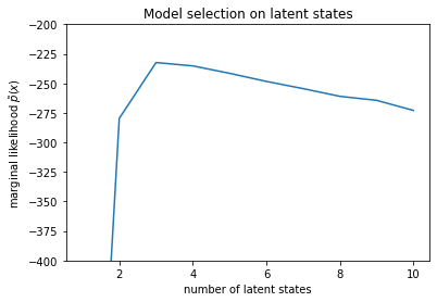
가능성을 조사하면 (근사치) 한계 가능성이 3-상태 모델을 선호하는 경향이 있음을 알 수 있습니다. 이것은 꽤 그럴듯해 보입니다. '진정한' 모델에는 4가지 상태가 있지만 데이터만 보면 3가지 상태 설명을 배제하기 어렵습니다.
또한 각 후보 모델에 맞는 비율을 추출할 수 있습니다.
rates = tf.exp(trainable_log_rates)
for i, learned_model_rates in enumerate(rates):
  print("rates for {}-state model: {}".format(i+1, learned_model_rates[:i+1]))
rates for 1-state model: [32.968506]
rates for 2-state model: [ 5.789209 47.948917]
rates for 3-state model: [ 2.841977 48.057507 17.958897]
rates for 4-state model: [ 2.8302798 49.585037  41.928406  17.351114 ]
rates for 5-state model: [17.399694  77.83679   41.975216  49.62771    2.8256145]
rates for 6-state model: [41.63677   77.20768   49.570934  49.557076  17.630419   2.8713436]
rates for 7-state model: [41.711704  76.405945  49.581184  49.561283  17.451889   2.8722699
 17.43608  ]
rates for 8-state model: [41.771793 75.41323  49.568714 49.591846 17.2523   17.247969 17.231388
  2.830598]
rates for 9-state model: [41.83378   74.50916   49.619488  49.622494   2.8369408 17.254414
 17.21532    2.5904858 17.252514 ]
rates for 10-state model: [4.1886074e+01 7.3912338e+01 4.1940136e+01 4.9652588e+01 2.8485537e+00
 1.7433832e+01 6.7564294e-02 1.9590002e+00 1.7430998e+01 7.8838937e-02]
그리고 각 모델이 데이터에 대해 제공하는 설명을 플로팅합니다.
most_probable_states = hmm.posterior_mode(observed_counts)
fig = plt.figure(figsize=(14, 12))
for i, learned_model_rates in enumerate(rates):
  ax = fig.add_subplot(4, 3, i+1)
  ax.plot(tf.gather(learned_model_rates, most_probable_states[i]), c='green', lw=3, label='inferred rate')
  ax.plot(observed_counts, c='black', alpha=0.3, label='observed counts')
  ax.set_ylabel("latent rate")
  ax.set_xlabel("time")
  ax.set_title("{}-state model".format(i+1))
  ax.legend(loc=4)
plt.tight_layout()
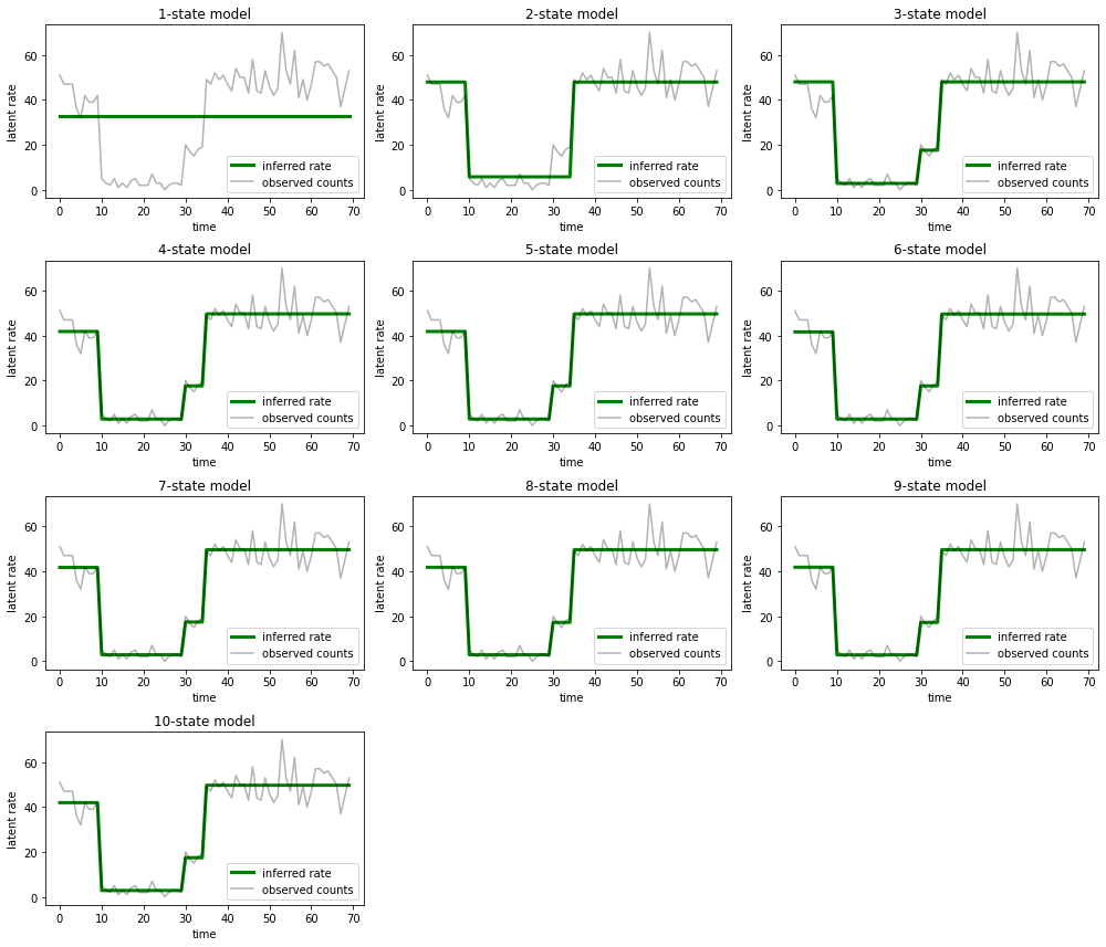
1-, 2-, (좀 더 미묘하게) 3-상태 모델이 어떻게 부적절한 설명을 제공하는지 쉽게 알 수 있습니다. 흥미롭게도 4개 상태 이상의 모든 모델은 본질적으로 동일한 설명을 제공합니다! 이것은 우리의 '데이터'가 비교적 깨끗하고 대체 설명의 여지가 거의 없기 때문일 수 있습니다. 더 지저분한 실제 데이터에서 더 높은 용량의 모델이 데이터에 점진적으로 더 나은 적합을 제공할 것으로 예상할 수 있으며, 일부 절충점은 개선된 적합도가 모델 복잡성보다 더 중요합니다.
확장
이 노트북의 모델은 여러 가지 방법으로 간단하게 확장할 수 있습니다. 예를 들어:
- 잠재 상태가 다른 확률을 갖도록 허용(일부 상태는 일반적이거나 희귀할 수 있음)
- 잠재 상태 간의 불균일한 전환 허용(예: 일반적으로 시스템 충돌 후 시스템 재부팅이 뒤따른다는 것을 학습하려면 일반적으로 일정 기간 동안 우수한 성능을 발휘하는 등)
- 다른 방출 모델은, 예를 들어
NegativeBinomial같은 계수 데이터, 또는 연속 분포의 분산을 다양한 모델링하는Normal실수 데이터.