| | |  Xem nguồn trên GitHub Xem nguồn trên GitHub | |
Sổ tay này trình bày việc sử dụng các công cụ suy luận gần đúng TFP để kết hợp mô hình quan sát (không phải Gaussian) khi phù hợp và dự báo với các mô hình chuỗi thời gian cấu trúc (STS). Trong ví dụ này, chúng tôi sẽ sử dụng mô hình quan sát Poisson để làm việc với dữ liệu đếm rời rạc.
import time
import matplotlib.pyplot as plt
import numpy as np

import tensorflow.compat.v2 as tf
import tensorflow_probability as tfp

from tensorflow_probability import bijectors as tfb
from tensorflow_probability import distributions as tfd

tf.enable_v2_behavior()
Dữ liệu tổng hợp
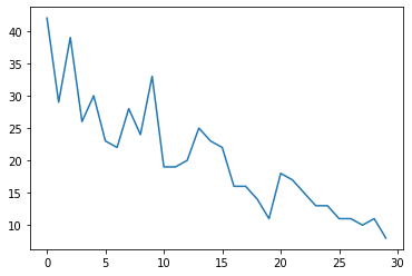
Đầu tiên, chúng tôi sẽ tạo một số dữ liệu đếm tổng hợp:
num_timesteps = 30
observed_counts = np.round(3 + np.random.lognormal(np.log(np.linspace(
    num_timesteps, 5, num=num_timesteps)), 0.20, size=num_timesteps))
observed_counts = observed_counts.astype(np.float32)
plt.plot(observed_counts)
[<matplotlib.lines.Line2D at 0x7f940ae958d0>]
Mô hình
Chúng tôi sẽ chỉ định một mô hình đơn giản với xu hướng tuyến tính đi bộ ngẫu nhiên:
def build_model(approximate_unconstrained_rates):
  trend = tfp.sts.LocalLinearTrend(
      observed_time_series=approximate_unconstrained_rates)
  return tfp.sts.Sum([trend],
                     observed_time_series=approximate_unconstrained_rates)
Thay vì hoạt động trên chuỗi thời gian được quan sát, mô hình này sẽ hoạt động trên chuỗi các tham số tốc độ Poisson chi phối các quan sát.
Vì tỷ lệ Poisson phải dương, chúng tôi sẽ sử dụng bijector để chuyển đổi mô hình STS có giá trị thực thành một phân phối trên các giá trị dương. Các Softplus chuyển đổi \(y = \log(1 + \exp(x))\) là một lựa chọn tất yếu, vì nó là gần như tuyến tính cho các giá trị tích cực, nhưng sự lựa chọn khác như Exp (mà biến đổi bước đi ngẫu nhiên bình thường thành một bước đi ngẫu nhiên lognormal) cũng có thể.
positive_bijector = tfb.Softplus()  # Or tfb.Exp()

# Approximate the unconstrained Poisson rate just to set heuristic priors.
# We could avoid this by passing explicit priors on all model params.
approximate_unconstrained_rates = positive_bijector.inverse(
    tf.convert_to_tensor(observed_counts) + 0.01)
sts_model = build_model(approximate_unconstrained_rates)
Để sử dụng suy luận gần đúng cho mô hình quan sát không phải Gaussian, chúng tôi sẽ mã hóa mô hình STS dưới dạng Phân phối chung TFP. Các biến ngẫu nhiên trong phân phối chung này là các tham số của mô hình STS, chuỗi thời gian của tỷ lệ Poisson tiềm ẩn và số lượng quan sát được.
def sts_with_poisson_likelihood_model():
  # Encode the parameters of the STS model as random variables.
  param_vals = []
  for param in sts_model.parameters:
    param_val = yield param.prior
    param_vals.append(param_val)

  # Use the STS model to encode the log- (or inverse-softplus)
  # rate of a Poisson.
  unconstrained_rate = yield sts_model.make_state_space_model(
      num_timesteps, param_vals)
  rate = positive_bijector.forward(unconstrained_rate[..., 0])
  observed_counts = yield tfd.Poisson(rate, name='observed_counts')

model = tfd.JointDistributionCoroutineAutoBatched(sts_with_poisson_likelihood_model)
Chuẩn bị cho suy luận
Chúng tôi muốn suy ra các đại lượng không quan sát được trong mô hình, với số lượng quan sát được. Đầu tiên, chúng tôi điều chỉnh mật độ nhật ký chung trên các số đếm được quan sát.
pinned_model = model.experimental_pin(observed_counts=observed_counts)
Chúng ta cũng sẽ cần một bijector hạn chế để đảm bảo rằng suy luận tôn trọng các ràng buộc đối với các tham số của mô hình STS (ví dụ: thang đo phải là số dương).
constraining_bijector = pinned_model.experimental_default_event_space_bijector()
Suy luận với HMC
Chúng tôi sẽ sử dụng HMC (cụ thể là NUTS) để lấy mẫu từ phía sau chung trên các thông số mô hình và tỷ lệ tiềm ẩn.
Điều này sẽ chậm hơn đáng kể so với việc lắp mô hình STS tiêu chuẩn với HMC, vì ngoài các tham số (số lượng tương đối nhỏ) của mô hình, chúng tôi cũng phải suy ra toàn bộ chuỗi tỷ lệ Poisson. Vì vậy, chúng tôi sẽ chạy cho một số bước tương đối nhỏ; đối với các ứng dụng mà chất lượng suy luận là quan trọng, có thể có ý nghĩa khi tăng các giá trị này hoặc chạy nhiều chuỗi.
Cấu hình bộ lấy mẫu
# Allow external control of sampling to reduce test runtimes.
num_results = 500 # @param { isTemplate: true}
num_results = int(num_results)

num_burnin_steps = 100 # @param { isTemplate: true}
num_burnin_steps = int(num_burnin_steps)
Đầu tiên chúng tôi chỉ định một sampler, và sau đó sử dụng sample_chain để chạy mà hạt nhân lấy mẫu để mẫu sản phẩm.
sampler = tfp.mcmc.TransformedTransitionKernel(
    tfp.mcmc.NoUTurnSampler(
        target_log_prob_fn=pinned_model.unnormalized_log_prob,
        step_size=0.1),
    bijector=constraining_bijector)

adaptive_sampler = tfp.mcmc.DualAveragingStepSizeAdaptation(
    inner_kernel=sampler,
    num_adaptation_steps=int(0.8 * num_burnin_steps),
    target_accept_prob=0.75)

initial_state = constraining_bijector.forward(
    type(pinned_model.event_shape)(
        *(tf.random.normal(part_shape)
          for part_shape in constraining_bijector.inverse_event_shape(
              pinned_model.event_shape))))
# Speed up sampling by tracing with `tf.function`.
@tf.function(autograph=False, jit_compile=True)
def do_sampling():
  return tfp.mcmc.sample_chain(
      kernel=adaptive_sampler,
      current_state=initial_state,
      num_results=num_results,
      num_burnin_steps=num_burnin_steps,
      trace_fn=None)

t0 = time.time()
samples = do_sampling()
t1 = time.time()
print("Inference ran in {:.2f}s.".format(t1-t0))
Inference ran in 24.83s.
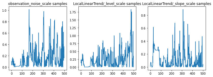
Chúng ta có thể kiểm tra sự tỉnh táo bằng cách kiểm tra các dấu vết tham số. Trong trường hợp này, họ dường như đã khám phá nhiều lời giải thích cho dữ liệu, điều này là tốt, mặc dù nhiều mẫu hơn sẽ hữu ích để đánh giá mức độ trộn lẫn của chuỗi.
f = plt.figure(figsize=(12, 4))
for i, param in enumerate(sts_model.parameters):
  ax = f.add_subplot(1, len(sts_model.parameters), i + 1)
  ax.plot(samples[i])
  ax.set_title("{} samples".format(param.name))
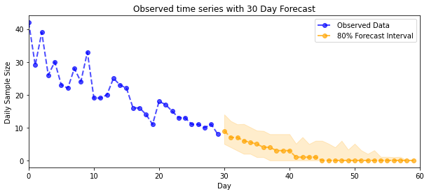
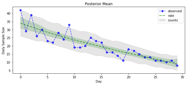
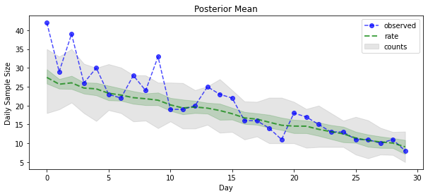
Bây giờ cho phần thưởng: chúng ta hãy xem hậu quả của tỷ lệ Poisson! Chúng tôi cũng sẽ vẽ biểu đồ khoảng thời gian dự đoán 80% trên các số đếm được quan sát và có thể kiểm tra xem khoảng này có chứa khoảng 80% số lượng mà chúng tôi thực sự quan sát được hay không.
param_samples = samples[:-1]
unconstrained_rate_samples = samples[-1][..., 0]
rate_samples = positive_bijector.forward(unconstrained_rate_samples)

plt.figure(figsize=(10, 4))
mean_lower, mean_upper = np.percentile(rate_samples, [10, 90], axis=0)
pred_lower, pred_upper = np.percentile(np.random.poisson(rate_samples),
                                       [10, 90], axis=0)

_ = plt.plot(observed_counts, color="blue", ls='--', marker='o', label='observed', alpha=0.7)
_ = plt.plot(np.mean(rate_samples, axis=0), label='rate', color="green", ls='dashed', lw=2, alpha=0.7)
_ = plt.fill_between(np.arange(0, 30), mean_lower, mean_upper, color='green', alpha=0.2)
_ = plt.fill_between(np.arange(0, 30), pred_lower, pred_upper, color='grey', label='counts', alpha=0.2)
plt.xlabel("Day")
plt.ylabel("Daily Sample Size")
plt.title("Posterior Mean")
plt.legend()
<matplotlib.legend.Legend at 0x7f93ffd35550>
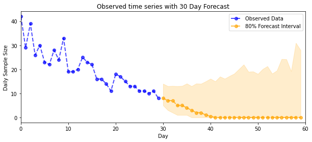
Dự báo
Để dự báo số lượng quan sát được, chúng tôi sẽ sử dụng các công cụ STS tiêu chuẩn để xây dựng phân phối dự báo theo tỷ lệ tiềm ẩn (trong không gian không bị giới hạn, một lần nữa vì STS được thiết kế để lập mô hình dữ liệu có giá trị thực), sau đó chuyển các dự báo được lấy mẫu thông qua quan sát Poisson mô hình:
def sample_forecasted_counts(sts_model, posterior_latent_rates,
                             posterior_params, num_steps_forecast,
                             num_sampled_forecasts):

  # Forecast the future latent unconstrained rates, given the inferred latent
  # unconstrained rates and parameters.
  unconstrained_rates_forecast_dist = tfp.sts.forecast(sts_model,
    observed_time_series=unconstrained_rate_samples,
    parameter_samples=posterior_params,
    num_steps_forecast=num_steps_forecast)

  # Transform the forecast to positive-valued Poisson rates.
  rates_forecast_dist = tfd.TransformedDistribution(
      unconstrained_rates_forecast_dist,
      positive_bijector)

  # Sample from the forecast model following the chain rule:
  # P(counts) = P(counts | latent_rates)P(latent_rates)
  sampled_latent_rates = rates_forecast_dist.sample(num_sampled_forecasts)
  sampled_forecast_counts = tfd.Poisson(rate=sampled_latent_rates).sample()

  return sampled_forecast_counts, sampled_latent_rates

forecast_samples, rate_samples = sample_forecasted_counts(
   sts_model,
   posterior_latent_rates=unconstrained_rate_samples,
   posterior_params=param_samples,
   # Days to forecast:
   num_steps_forecast=30,
   num_sampled_forecasts=100)
forecast_samples = np.squeeze(forecast_samples)
def plot_forecast_helper(data, forecast_samples, CI=90):
  """Plot the observed time series alongside the forecast."""
  plt.figure(figsize=(10, 4))
  forecast_median = np.median(forecast_samples, axis=0)

  num_steps = len(data)
  num_steps_forecast = forecast_median.shape[-1]

  plt.plot(np.arange(num_steps), data, lw=2, color='blue', linestyle='--', marker='o',
           label='Observed Data', alpha=0.7)

  forecast_steps = np.arange(num_steps, num_steps+num_steps_forecast)

  CI_interval = [(100 - CI)/2, 100 - (100 - CI)/2]
  lower, upper = np.percentile(forecast_samples, CI_interval, axis=0)

  plt.plot(forecast_steps, forecast_median, lw=2, ls='--', marker='o', color='orange',
           label=str(CI) + '% Forecast Interval', alpha=0.7)
  plt.fill_between(forecast_steps,
                   lower,
                   upper, color='orange', alpha=0.2)

  plt.xlim([0, num_steps+num_steps_forecast])
  ymin, ymax = min(np.min(forecast_samples), np.min(data)), max(np.max(forecast_samples), np.max(data))
  yrange = ymax-ymin
  plt.title("{}".format('Observed time series with ' + str(num_steps_forecast) + ' Day Forecast'))
  plt.xlabel('Day')
  plt.ylabel('Daily Sample Size')
  plt.legend()
plot_forecast_helper(observed_counts, forecast_samples, CI=80)
Suy luận VI
Variational suy luận có thể có vấn đề khi suy luận một loạt đầy đủ thời gian, như đếm xấp xỉ của chúng tôi (như trái ngược với chỉ các thông số của một chuỗi thời gian, như trong STS mô hình tiêu chuẩn). Giả định tiêu chuẩn rằng các biến có hậu kiểm độc lập là khá sai, vì mỗi bước thời gian đều có tương quan với các biến lân cận của nó, điều này có thể dẫn đến việc đánh giá thấp độ không chắc chắn. Vì lý do này, HMC có thể là lựa chọn tốt hơn để suy luận gần đúng trên chuỗi thời gian đầy đủ. Tuy nhiên, VI có thể nhanh hơn một chút và có thể hữu ích cho việc tạo mẫu mô hình hoặc trong các trường hợp mà hiệu suất của nó có thể được chứng minh theo kinh nghiệm là 'đủ tốt'.
Để phù hợp với mô hình của chúng tôi với VI, chúng tôi chỉ cần xây dựng và tối ưu hóa phần sau thay thế:
surrogate_posterior = tfp.experimental.vi.build_factored_surrogate_posterior(
    event_shape=pinned_model.event_shape,
    bijector=constraining_bijector)
# Allow external control of optimization to reduce test runtimes.
num_variational_steps = 1000 # @param { isTemplate: true}
num_variational_steps = int(num_variational_steps)

t0 = time.time()
losses = tfp.vi.fit_surrogate_posterior(pinned_model.unnormalized_log_prob,
                                        surrogate_posterior,
                                        optimizer=tf.optimizers.Adam(0.1),
                                        num_steps=num_variational_steps)
t1 = time.time()
print("Inference ran in {:.2f}s.".format(t1-t0))
Inference ran in 11.37s.
plt.plot(losses)
plt.title("Variational loss")
_ = plt.xlabel("Steps")

posterior_samples = surrogate_posterior.sample(50)
param_samples = posterior_samples[:-1]
unconstrained_rate_samples = posterior_samples[-1][..., 0]
rate_samples = positive_bijector.forward(unconstrained_rate_samples)

plt.figure(figsize=(10, 4))
mean_lower, mean_upper = np.percentile(rate_samples, [10, 90], axis=0)
pred_lower, pred_upper = np.percentile(
    np.random.poisson(rate_samples), [10, 90], axis=0)

_ = plt.plot(observed_counts, color='blue', ls='--', marker='o',
             label='observed', alpha=0.7)
_ = plt.plot(np.mean(rate_samples, axis=0), label='rate', color='green',
             ls='dashed', lw=2, alpha=0.7)
_ = plt.fill_between(
    np.arange(0, 30), mean_lower, mean_upper, color='green', alpha=0.2)
_ = plt.fill_between(np.arange(0, 30), pred_lower, pred_upper, color='grey',
    label='counts', alpha=0.2)
plt.xlabel('Day')
plt.ylabel('Daily Sample Size')
plt.title('Posterior Mean')
plt.legend()
<matplotlib.legend.Legend at 0x7f93ff4735c0>
forecast_samples, rate_samples = sample_forecasted_counts(
   sts_model,
   posterior_latent_rates=unconstrained_rate_samples,
   posterior_params=param_samples,
   # Days to forecast:
   num_steps_forecast=30,
   num_sampled_forecasts=100)
forecast_samples = np.squeeze(forecast_samples)
plot_forecast_helper(observed_counts, forecast_samples, CI=80)