מחברת זו ממחישה שתי דוגמאות להתאמת מודלים מבניים של סדרות זמן לסדרות זמן ושימוש בהם ליצירת תחזיות והסברים.
| | |  צפה במקור ב-GitHub צפה במקור ב-GitHub | |
תלות ודרישות מוקדמות
ייבוא והגדרות
%matplotlib inline
import matplotlib as mpl
from matplotlib import pylab as plt
import matplotlib.dates as mdates
import seaborn as sns

import collections

import numpy as np
import tensorflow.compat.v2 as tf
import tensorflow_probability as tfp

from tensorflow_probability import distributions as tfd
from tensorflow_probability import sts

tf.enable_v2_behavior()
הפוך דברים מהר!
לפני שנצלול פנימה, בואו נוודא שאנחנו משתמשים ב-GPU עבור הדגמה זו.
כדי לעשות זאת, בחר "זמן ריצה" -> "שנה סוג זמן ריצה" -> "מאיץ חומרה" -> "GPU".
הקטע הבא יאמת שיש לנו גישה ל-GPU.
if tf.test.gpu_device_name() != '/device:GPU:0':
  print('WARNING: GPU device not found.')
else:
  print('SUCCESS: Found GPU: {}'.format(tf.test.gpu_device_name()))
SUCCESS: Found GPU: /device:GPU:0
הגדרת מזימות
שיטות עוזר לשרטוט סדרות זמן ותחזיות.
from pandas.plotting import register_matplotlib_converters
register_matplotlib_converters()

sns.set_context("notebook", font_scale=1.)
sns.set_style("whitegrid")
%config InlineBackend.figure_format = 'retina'
def plot_forecast(x, y,
                  forecast_mean, forecast_scale, forecast_samples,
                  title, x_locator=None, x_formatter=None):
  """Plot a forecast distribution against the 'true' time series."""
  colors = sns.color_palette()
  c1, c2 = colors[0], colors[1]
  fig = plt.figure(figsize=(12, 6))
  ax = fig.add_subplot(1, 1, 1)

  num_steps = len(y)
  num_steps_forecast = forecast_mean.shape[-1]
  num_steps_train = num_steps - num_steps_forecast


  ax.plot(x, y, lw=2, color=c1, label='ground truth')

  forecast_steps = np.arange(
      x[num_steps_train],
      x[num_steps_train]+num_steps_forecast,
      dtype=x.dtype)

  ax.plot(forecast_steps, forecast_samples.T, lw=1, color=c2, alpha=0.1)

  ax.plot(forecast_steps, forecast_mean, lw=2, ls='--', color=c2,
           label='forecast')
  ax.fill_between(forecast_steps,
                   forecast_mean-2*forecast_scale,
                   forecast_mean+2*forecast_scale, color=c2, alpha=0.2)

  ymin, ymax = min(np.min(forecast_samples), np.min(y)), max(np.max(forecast_samples), np.max(y))
  yrange = ymax-ymin
  ax.set_ylim([ymin - yrange*0.1, ymax + yrange*0.1])
  ax.set_title("{}".format(title))
  ax.legend()

  if x_locator is not None:
    ax.xaxis.set_major_locator(x_locator)
    ax.xaxis.set_major_formatter(x_formatter)
    fig.autofmt_xdate()

  return fig, ax
def plot_components(dates,
                    component_means_dict,
                    component_stddevs_dict,
                    x_locator=None,
                    x_formatter=None):
  """Plot the contributions of posterior components in a single figure."""
  colors = sns.color_palette()
  c1, c2 = colors[0], colors[1]

  axes_dict = collections.OrderedDict()
  num_components = len(component_means_dict)
  fig = plt.figure(figsize=(12, 2.5 * num_components))
  for i, component_name in enumerate(component_means_dict.keys()):
    component_mean = component_means_dict[component_name]
    component_stddev = component_stddevs_dict[component_name]

    ax = fig.add_subplot(num_components,1,1+i)
    ax.plot(dates, component_mean, lw=2)
    ax.fill_between(dates,
                     component_mean-2*component_stddev,
                     component_mean+2*component_stddev,
                     color=c2, alpha=0.5)
    ax.set_title(component_name)
    if x_locator is not None:
      ax.xaxis.set_major_locator(x_locator)
      ax.xaxis.set_major_formatter(x_formatter)
    axes_dict[component_name] = ax
  fig.autofmt_xdate()
  fig.tight_layout()
  return fig, axes_dict
def plot_one_step_predictive(dates, observed_time_series,
                             one_step_mean, one_step_scale,
                             x_locator=None, x_formatter=None):
  """Plot a time series against a model's one-step predictions."""

  colors = sns.color_palette()
  c1, c2 = colors[0], colors[1]

  fig=plt.figure(figsize=(12, 6))
  ax = fig.add_subplot(1,1,1)
  num_timesteps = one_step_mean.shape[-1]
  ax.plot(dates, observed_time_series, label="observed time series", color=c1)
  ax.plot(dates, one_step_mean, label="one-step prediction", color=c2)
  ax.fill_between(dates,
                  one_step_mean - one_step_scale,
                  one_step_mean + one_step_scale,
                  alpha=0.1, color=c2)
  ax.legend()

  if x_locator is not None:
    ax.xaxis.set_major_locator(x_locator)
    ax.xaxis.set_major_formatter(x_formatter)
    fig.autofmt_xdate()
  fig.tight_layout()
  return fig, ax
שיא CO2 במאונה לואה
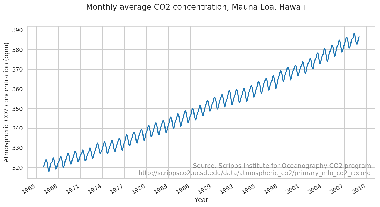
נדגים התאמת מודל לקריאות CO2 באטמוספירה ממצפה הכוכבים מאונה לואה.
נתונים
# CO2 readings from Mauna Loa observatory, monthly beginning January 1966
# Original source: http://scrippsco2.ucsd.edu/data/atmospheric_co2/primary_mlo_co2_record
co2_by_month = np.array('320.62,321.60,322.39,323.70,324.08,323.75,322.38,320.36,318.64,318.10,319.78,321.03,322.33,322.50,323.04,324.42,325.00,324.09,322.54,320.92,319.25,319.39,320.73,321.96,322.57,323.15,323.89,325.02,325.57,325.36,324.14,322.11,320.33,320.25,321.32,322.89,324.00,324.42,325.63,326.66,327.38,326.71,325.88,323.66,322.38,321.78,322.85,324.12,325.06,325.98,326.93,328.14,328.08,327.67,326.34,324.69,323.10,323.06,324.01,325.13,326.17,326.68,327.17,327.79,328.92,328.57,327.36,325.43,323.36,323.56,324.80,326.01,326.77,327.63,327.75,329.73,330.07,329.09,328.04,326.32,324.84,325.20,326.50,327.55,328.55,329.56,330.30,331.50,332.48,332.07,330.87,329.31,327.51,327.18,328.16,328.64,329.35,330.71,331.48,332.65,333.09,332.25,331.18,329.39,327.43,327.37,328.46,329.57,330.40,331.40,332.04,333.31,333.97,333.60,331.90,330.06,328.56,328.34,329.49,330.76,331.75,332.56,333.50,334.58,334.88,334.33,333.05,330.94,329.30,328.94,330.31,331.68,332.93,333.42,334.70,336.07,336.75,336.27,334.92,332.75,331.59,331.16,332.40,333.85,334.97,335.38,336.64,337.76,338.01,337.89,336.54,334.68,332.76,332.55,333.92,334.95,336.23,336.76,337.96,338.88,339.47,339.29,337.73,336.09,333.92,333.86,335.29,336.73,338.01,338.36,340.07,340.77,341.47,341.17,339.56,337.60,335.88,336.02,337.10,338.21,339.24,340.48,341.38,342.51,342.91,342.25,340.49,338.43,336.69,336.86,338.36,339.61,340.75,341.61,342.70,343.57,344.14,343.35,342.06,339.81,337.98,337.86,339.26,340.49,341.38,342.52,343.10,344.94,345.76,345.32,343.98,342.38,339.87,339.99,341.15,342.99,343.70,344.50,345.28,347.06,347.43,346.80,345.39,343.28,341.07,341.35,342.98,344.22,344.97,345.99,347.42,348.35,348.93,348.25,346.56,344.67,343.09,342.80,344.24,345.56,346.30,346.95,347.85,349.55,350.21,349.55,347.94,345.90,344.85,344.17,345.66,346.90,348.02,348.48,349.42,350.99,351.85,351.26,349.51,348.10,346.45,346.36,347.81,348.96,350.43,351.73,352.22,353.59,354.22,353.79,352.38,350.43,348.73,348.88,350.07,351.34,352.76,353.07,353.68,355.42,355.67,355.12,353.90,351.67,349.80,349.99,351.30,352.52,353.66,354.70,355.38,356.20,357.16,356.23,354.81,352.91,350.96,351.18,352.83,354.21,354.72,355.75,357.16,358.60,359.34,358.24,356.17,354.02,352.15,352.21,353.75,354.99,355.99,356.72,357.81,359.15,359.66,359.25,357.02,355.00,353.01,353.31,354.16,355.40,356.70,357.17,358.38,359.46,360.28,359.60,357.57,355.52,353.69,353.99,355.34,356.80,358.37,358.91,359.97,361.26,361.69,360.94,359.55,357.48,355.84,356.00,357.58,359.04,359.97,361.00,361.64,363.45,363.80,363.26,361.89,359.45,358.05,357.75,359.56,360.70,362.05,363.24,364.02,364.71,365.41,364.97,363.65,361.48,359.45,359.61,360.76,362.33,363.18,363.99,364.56,366.36,366.80,365.63,364.47,362.50,360.19,360.78,362.43,364.28,365.33,366.15,367.31,368.61,369.30,368.88,367.64,365.78,363.90,364.23,365.46,366.97,368.15,368.87,369.59,371.14,371.00,370.35,369.27,366.93,364.64,365.13,366.68,368.00,369.14,369.46,370.51,371.66,371.83,371.69,370.12,368.12,366.62,366.73,368.29,369.53,370.28,371.50,372.12,372.86,374.02,373.31,371.62,369.55,367.96,368.09,369.68,371.24,372.44,373.08,373.52,374.85,375.55,375.40,374.02,371.48,370.70,370.25,372.08,373.78,374.68,375.62,376.11,377.65,378.35,378.13,376.61,374.48,372.98,373.00,374.35,375.69,376.79,377.36,378.39,380.50,380.62,379.55,377.76,375.83,374.05,374.22,375.84,377.44,378.34,379.61,380.08,382.05,382.24,382.08,380.67,378.67,376.42,376.80,378.31,379.96,381.37,382.02,382.56,384.37,384.92,384.03,382.28,380.48,378.81,379.06,380.14,381.66,382.58,383.71,384.34,386.23,386.41,385.87,384.45,381.84,380.86,380.86,382.36,383.61,385.07,385.84,385.83,386.77,388.51,388.05,386.25,384.08,383.09,382.78,384.01,385.11,386.65,387.12,388.52,389.57,390.16,389.62,388.07,386.08,384.65,384.33,386.05,387.49,388.55,390.07,391.01,392.38,393.22,392.24,390.33,388.52,386.84,387.16,388.67,389.81,391.30,391.92,392.45,393.37,394.28,393.69,392.59,390.21,389.00,388.93,390.24,391.80,393.07,393.35,394.36,396.43,396.87,395.88,394.52,392.54,391.13,391.01,392.95,394.34,395.61,396.85,397.26,398.35,399.98,398.87,397.37,395.41,393.39,393.70,395.19,396.82,397.92,398.10,399.47,401.33,401.88,401.31,399.07,397.21,395.40,395.65,397.23,398.79,399.85,400.31,401.51,403.45,404.10,402.88,401.61,399.00,397.50,398.28,400.24,401.89,402.65,404.16,404.85,407.57,407.66,407.00,404.50,402.24,401.01,401.50,403.64,404.55,406.07,406.64,407.06,408.95,409.91,409.12,407.20,405.24,403.27,403.64,405.17,406.75,408.05,408.34,409.25,410.30,411.30,410.88,408.90,407.10,405.59,405.99,408.12,409.23,410.92'.split(',')).astype(np.float32)

co2_by_month = co2_by_month
num_forecast_steps = 12 * 10 # Forecast the final ten years, given previous data
co2_by_month_training_data = co2_by_month[:-num_forecast_steps]

co2_dates = np.arange("1966-01", "2019-02", dtype="datetime64[M]")
co2_loc = mdates.YearLocator(3)
co2_fmt = mdates.DateFormatter('%Y')
fig = plt.figure(figsize=(12, 6))
ax = fig.add_subplot(1, 1, 1)
ax.plot(co2_dates[:-num_forecast_steps], co2_by_month_training_data, lw=2, label="training data")
ax.xaxis.set_major_locator(co2_loc)
ax.xaxis.set_major_formatter(co2_fmt)
ax.set_ylabel("Atmospheric CO2 concentration (ppm)")
ax.set_xlabel("Year")
fig.suptitle("Monthly average CO2 concentration, Mauna Loa, Hawaii",
             fontsize=15)
ax.text(0.99, .02,
        "Source: Scripps Institute for Oceanography CO2 program\nhttp://scrippsco2.ucsd.edu/data/atmospheric_co2/primary_mlo_co2_record",
        transform=ax.transAxes,
        horizontalalignment="right",
        alpha=0.5)
fig.autofmt_xdate()
דגם והתאמה
אנו נדגמן את הסדרה הזו עם מגמה ליניארית מקומית, בתוספת אפקט עונתי של חודש בשנה.
def build_model(observed_time_series):
  trend = sts.LocalLinearTrend(observed_time_series=observed_time_series)
  seasonal = tfp.sts.Seasonal(
      num_seasons=12, observed_time_series=observed_time_series)
  model = sts.Sum([trend, seasonal], observed_time_series=observed_time_series)
  return model
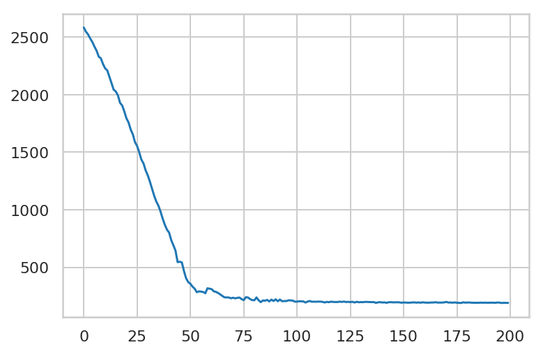
אנו נתאים את המודל באמצעות הסקת מסקנות וריאציות. זה כרוך בהפעלת אופטימיזציה כדי למזער פונקציית אובדן וריאציה, ה-Reference Lower bound (ELBO). זה מתאים לסט של התפלגויות אחוריות משוערות עבור הפרמטרים (בפועל אנו מניחים שאלו הם נורמלים עצמאיים שהומרו למרחב התמיכה של כל פרמטר).
שיטות החיזוי tfp.sts דורשות דגימות אחוריות כקלט, אז נסיים על ידי ציור של אוסף דגימות מהחלק האחורי.
co2_model = build_model(co2_by_month_training_data)

# Build the variational surrogate posteriors `qs`.
variational_posteriors = tfp.sts.build_factored_surrogate_posterior(
    model=co2_model)
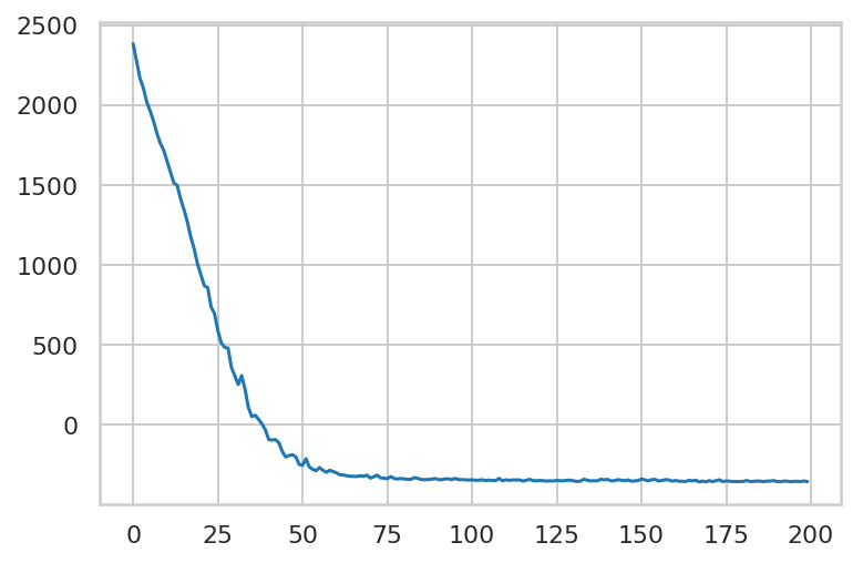
צמצם את ההפסד הווריאציוני.
# Allow external control of optimization to reduce test runtimes.
num_variational_steps = 200 # @param { isTemplate: true}
num_variational_steps = int(num_variational_steps)

# Build and optimize the variational loss function.
elbo_loss_curve = tfp.vi.fit_surrogate_posterior(
    target_log_prob_fn=co2_model.joint_distribution(
        observed_time_series=co2_by_month_training_data).log_prob,
    surrogate_posterior=variational_posteriors,
    optimizer=tf.optimizers.Adam(learning_rate=0.1),
    num_steps=num_variational_steps,
    jit_compile=True)

plt.plot(elbo_loss_curve)
plt.show()

# Draw samples from the variational posterior.
q_samples_co2_ = variational_posteriors.sample(50)
WARNING:tensorflow:From /usr/local/lib/python3.6/dist-packages/tensorflow_core/python/ops/linalg/linear_operator_diag.py:166: calling LinearOperator.__init__ (from tensorflow.python.ops.linalg.linear_operator) with graph_parents is deprecated and will be removed in a future version.
Instructions for updating:
Do not pass `graph_parents`.  They will  no longer be used.
print("Inferred parameters:")
for param in co2_model.parameters:
  print("{}: {} +- {}".format(param.name,
                              np.mean(q_samples_co2_[param.name], axis=0),
                              np.std(q_samples_co2_[param.name], axis=0)))
Inferred parameters:
observation_noise_scale: 0.17199112474918365 +- 0.009443143382668495
LocalLinearTrend/_level_scale: 0.17671072483062744 +- 0.01510554924607277
LocalLinearTrend/_slope_scale: 0.004302256740629673 +- 0.0018349259626120329
Seasonal/_drift_scale: 0.041069451719522476 +- 0.007772190496325493
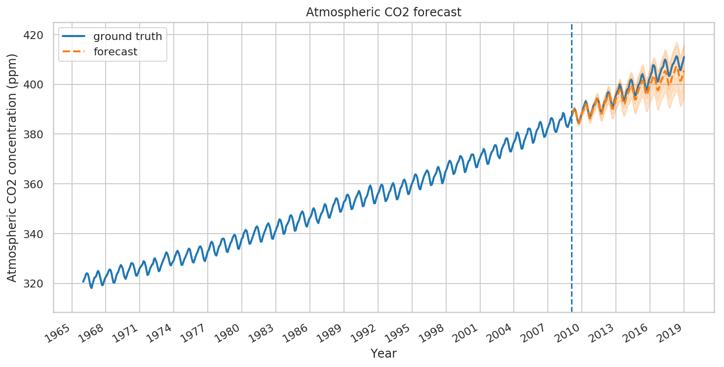
חיזוי וביקורת
כעת נשתמש במודל המותאם כדי לבנות תחזית. אנו פשוט קוראים tfp.sts.forecast , אשר מחזיר מופע TensorFlow Distribution המייצג את ההתפלגות החזויה על פני שלבי זמן עתידיים.
co2_forecast_dist = tfp.sts.forecast(
    co2_model,
    observed_time_series=co2_by_month_training_data,
    parameter_samples=q_samples_co2_,
    num_steps_forecast=num_forecast_steps)
בפרט, mean וה- stddev של התפלגות התחזית נותנים לנו תחזית עם אי ודאות שולית בכל צעד זמן, ונוכל גם לצייר דוגמאות של עתידים אפשריים.
num_samples=10

co2_forecast_mean, co2_forecast_scale, co2_forecast_samples = (
    co2_forecast_dist.mean().numpy()[..., 0],
    co2_forecast_dist.stddev().numpy()[..., 0],
    co2_forecast_dist.sample(num_samples).numpy()[..., 0])
fig, ax = plot_forecast(
    co2_dates, co2_by_month,
    co2_forecast_mean, co2_forecast_scale, co2_forecast_samples,
    x_locator=co2_loc,
    x_formatter=co2_fmt,
    title="Atmospheric CO2 forecast")
ax.axvline(co2_dates[-num_forecast_steps], linestyle="--")
ax.legend(loc="upper left")
ax.set_ylabel("Atmospheric CO2 concentration (ppm)")
ax.set_xlabel("Year")
fig.autofmt_xdate()
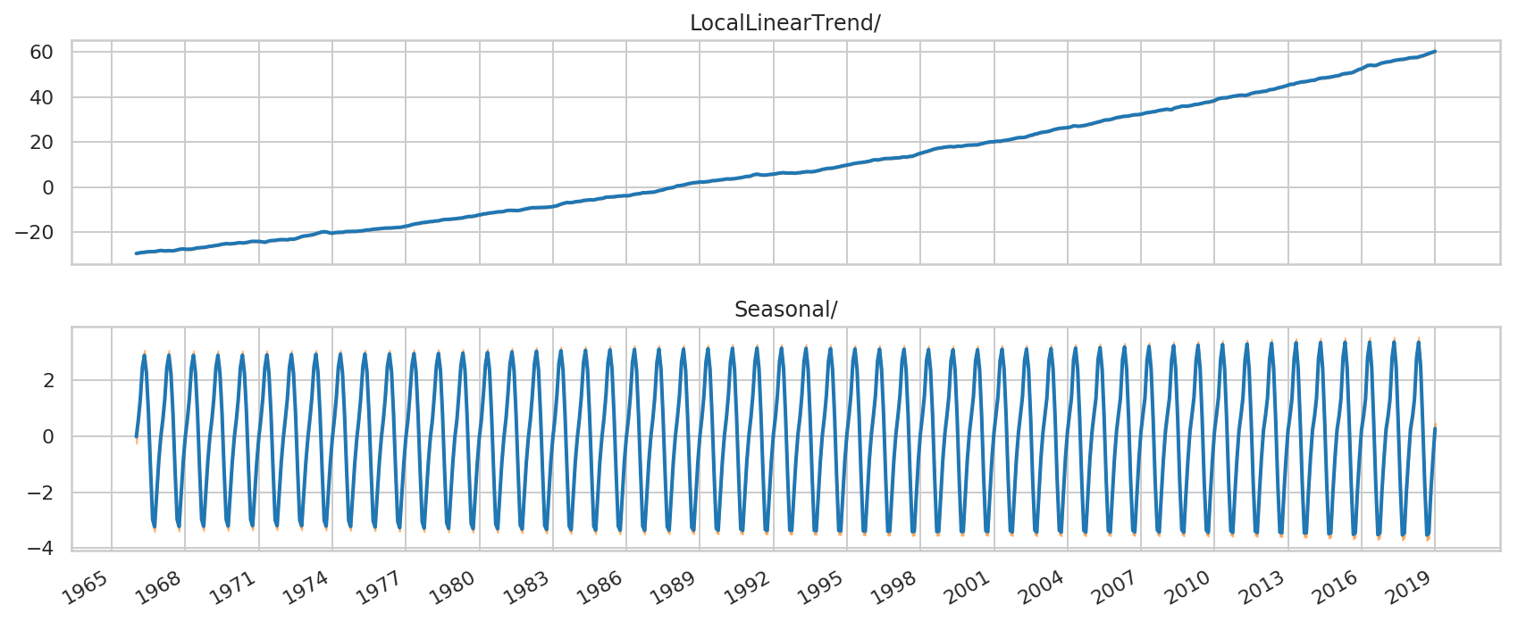
אנו יכולים להבין יותר את התאמת המודל על ידי פירוקו לתרומות של סדרות זמן בודדות:
# Build a dict mapping components to distributions over
# their contribution to the observed signal.
component_dists = sts.decompose_by_component(
    co2_model,
    observed_time_series=co2_by_month,
    parameter_samples=q_samples_co2_)
co2_component_means_, co2_component_stddevs_ = (
    {k.name: c.mean() for k, c in component_dists.items()},
    {k.name: c.stddev() for k, c in component_dists.items()})
_ = plot_components(co2_dates, co2_component_means_, co2_component_stddevs_,
                    x_locator=co2_loc, x_formatter=co2_fmt)
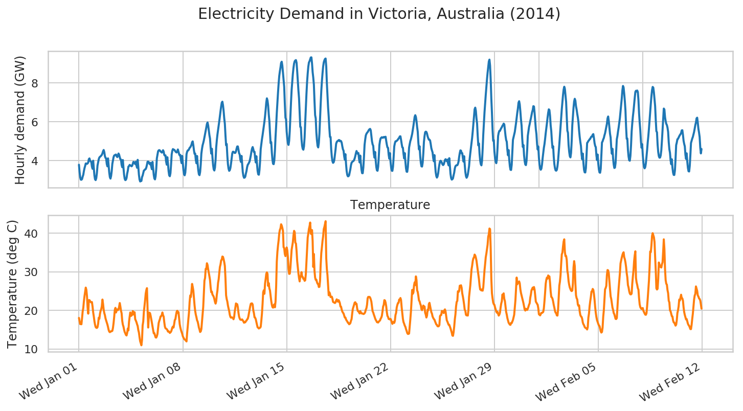
חיזוי ביקוש לחשמל
עכשיו בואו נשקול דוגמה מורכבת יותר: חיזוי הביקוש לחשמל בויקטוריה אוסטרליה.
ראשית, נבנה את מערך הנתונים:
# Victoria electricity demand dataset, as presented at
# https://otexts.com/fpp2/scatterplots.html
# and downloaded from https://github.com/robjhyndman/fpp2-package/blob/master/data/elecdaily.rda
# This series contains the first eight weeks (starting Jan 1). The original
# dataset was half-hourly data; here we've downsampled to hourly data by taking
# every other timestep.
demand_dates = np.arange('2014-01-01', '2014-02-26', dtype='datetime64[h]')
demand_loc = mdates.WeekdayLocator(byweekday=mdates.WE)
demand_fmt = mdates.DateFormatter('%a %b %d')

demand = np.array("3.794,3.418,3.152,3.026,3.022,3.055,3.180,3.276,3.467,3.620,3.730,3.858,3.851,3.839,3.861,3.912,4.082,4.118,4.011,3.965,3.932,3.693,3.585,4.001,3.623,3.249,3.047,3.004,3.104,3.361,3.749,3.910,4.075,4.165,4.202,4.225,4.265,4.301,4.381,4.484,4.552,4.440,4.233,4.145,4.116,3.831,3.712,4.121,3.764,3.394,3.159,3.081,3.216,3.468,3.838,4.012,4.183,4.269,4.280,4.310,4.315,4.233,4.188,4.263,4.370,4.308,4.182,4.075,4.057,3.791,3.667,4.036,3.636,3.283,3.073,3.003,3.023,3.113,3.335,3.484,3.697,3.723,3.786,3.763,3.748,3.714,3.737,3.828,3.937,3.929,3.877,3.829,3.950,3.756,3.638,4.045,3.682,3.283,3.036,2.933,2.956,2.959,3.157,3.236,3.370,3.493,3.516,3.555,3.570,3.656,3.792,3.950,3.953,3.926,3.849,3.813,3.891,3.683,3.562,3.936,3.602,3.271,3.085,3.041,3.201,3.570,4.123,4.307,4.481,4.533,4.545,4.524,4.470,4.457,4.418,4.453,4.539,4.473,4.301,4.260,4.276,3.958,3.796,4.180,3.843,3.465,3.246,3.203,3.360,3.808,4.328,4.509,4.598,4.562,4.566,4.532,4.477,4.442,4.424,4.486,4.579,4.466,4.338,4.270,4.296,4.034,3.877,4.246,3.883,3.520,3.306,3.252,3.387,3.784,4.335,4.465,4.529,4.536,4.589,4.660,4.691,4.747,4.819,4.950,4.994,4.798,4.540,4.352,4.370,4.047,3.870,4.245,3.848,3.509,3.302,3.258,3.419,3.809,4.363,4.605,4.793,4.908,5.040,5.204,5.358,5.538,5.708,5.888,5.966,5.817,5.571,5.321,5.141,4.686,4.367,4.618,4.158,3.771,3.555,3.497,3.646,4.053,4.687,5.052,5.342,5.586,5.808,6.038,6.296,6.548,6.787,6.982,7.035,6.855,6.561,6.181,5.899,5.304,4.795,4.862,4.264,3.820,3.588,3.481,3.514,3.632,3.857,4.116,4.375,4.462,4.460,4.422,4.398,4.407,4.480,4.621,4.732,4.735,4.572,4.385,4.323,4.069,3.940,4.247,3.821,3.416,3.220,3.124,3.132,3.181,3.337,3.469,3.668,3.788,3.834,3.894,3.964,4.109,4.275,4.472,4.623,4.703,4.594,4.447,4.459,4.137,3.913,4.231,3.833,3.475,3.302,3.279,3.519,3.975,4.600,4.864,5.104,5.308,5.542,5.759,6.005,6.285,6.617,6.993,7.207,7.095,6.839,6.387,6.048,5.433,4.904,4.959,4.425,4.053,3.843,3.823,4.017,4.521,5.229,5.802,6.449,6.975,7.506,7.973,8.359,8.596,8.794,9.030,9.090,8.885,8.525,8.147,7.797,6.938,6.215,6.123,5.495,5.140,4.896,4.812,5.024,5.536,6.293,7.000,7.633,8.030,8.459,8.768,9.000,9.113,9.155,9.173,9.039,8.606,8.095,7.617,7.208,6.448,5.740,5.718,5.106,4.763,4.610,4.566,4.737,5.204,5.988,6.698,7.438,8.040,8.484,8.837,9.052,9.114,9.214,9.307,9.313,9.006,8.556,8.275,7.911,7.077,6.348,6.175,5.455,5.041,4.759,4.683,4.908,5.411,6.199,6.923,7.593,8.090,8.497,8.843,9.058,9.159,9.231,9.253,8.852,7.994,7.388,6.735,6.264,5.690,5.227,5.220,4.593,4.213,3.984,3.891,3.919,4.031,4.287,4.558,4.872,4.963,5.004,5.017,5.057,5.064,5.000,5.023,5.007,4.923,4.740,4.586,4.517,4.236,4.055,4.337,3.848,3.473,3.273,3.198,3.204,3.252,3.404,3.560,3.767,3.896,3.934,3.972,3.985,4.032,4.122,4.239,4.389,4.499,4.406,4.356,4.396,4.106,3.914,4.265,3.862,3.546,3.360,3.359,3.649,4.180,4.813,5.086,5.301,5.384,5.434,5.470,5.529,5.582,5.618,5.636,5.561,5.291,5.000,4.840,4.767,4.364,4.160,4.452,4.011,3.673,3.503,3.483,3.695,4.213,4.810,5.028,5.149,5.182,5.208,5.179,5.190,5.220,5.202,5.216,5.232,5.019,4.828,4.686,4.657,4.304,4.106,4.389,3.955,3.643,3.489,3.479,3.695,4.187,4.732,4.898,4.997,5.001,5.022,5.052,5.094,5.143,5.178,5.250,5.255,5.075,4.867,4.691,4.665,4.352,4.121,4.391,3.966,3.615,3.437,3.430,3.666,4.149,4.674,4.851,5.011,5.105,5.242,5.378,5.576,5.790,6.030,6.254,6.340,6.253,6.039,5.736,5.490,4.936,4.580,4.742,4.230,3.895,3.712,3.700,3.906,4.364,4.962,5.261,5.463,5.495,5.477,5.394,5.250,5.159,5.081,5.083,5.038,4.857,4.643,4.526,4.428,4.141,3.975,4.290,3.809,3.423,3.217,3.132,3.192,3.343,3.606,3.803,3.963,3.998,3.962,3.894,3.814,3.776,3.808,3.914,4.033,4.079,4.027,3.974,4.057,3.859,3.759,4.132,3.716,3.325,3.111,3.030,3.046,3.096,3.254,3.390,3.606,3.718,3.755,3.768,3.768,3.834,3.957,4.199,4.393,4.532,4.516,4.380,4.390,4.142,3.954,4.233,3.795,3.425,3.209,3.124,3.177,3.288,3.498,3.715,4.092,4.383,4.644,4.909,5.184,5.518,5.889,6.288,6.643,6.729,6.567,6.179,5.903,5.278,4.788,4.885,4.363,4.011,3.823,3.762,3.998,4.598,5.349,5.898,6.487,6.941,7.381,7.796,8.185,8.522,8.825,9.103,9.198,8.889,8.174,7.214,6.481,5.611,5.026,5.052,4.484,4.148,3.955,3.873,4.060,4.626,5.272,5.441,5.535,5.534,5.610,5.671,5.724,5.793,5.838,5.908,5.868,5.574,5.276,5.065,4.976,4.554,4.282,4.547,4.053,3.720,3.536,3.524,3.792,4.420,5.075,5.208,5.344,5.482,5.701,5.936,6.210,6.462,6.683,6.979,7.059,6.893,6.535,6.121,5.797,5.152,4.705,4.805,4.272,3.975,3.805,3.775,3.996,4.535,5.275,5.509,5.730,5.870,6.034,6.175,6.340,6.500,6.603,6.804,6.787,6.460,6.043,5.627,5.367,4.866,4.575,4.728,4.157,3.795,3.607,3.537,3.596,3.803,4.125,4.398,4.660,4.853,5.115,5.412,5.669,5.930,6.216,6.466,6.641,6.605,6.316,5.821,5.520,5.016,4.657,4.746,4.197,3.823,3.613,3.505,3.488,3.532,3.716,4.011,4.421,4.836,5.296,5.766,6.233,6.646,7.011,7.380,7.660,7.804,7.691,7.364,7.019,6.260,5.545,5.437,4.806,4.457,4.235,4.172,4.396,5.002,5.817,6.266,6.732,7.049,7.184,7.085,6.798,6.632,6.408,6.218,5.968,5.544,5.217,4.964,4.758,4.328,4.074,4.367,3.883,3.536,3.404,3.396,3.624,4.271,4.916,4.953,5.016,5.048,5.106,5.124,5.200,5.244,5.242,5.341,5.368,5.166,4.910,4.762,4.700,4.276,4.035,4.318,3.858,3.550,3.399,3.382,3.590,4.261,4.937,4.994,5.094,5.168,5.303,5.410,5.571,5.740,5.900,6.177,6.274,6.039,5.700,5.389,5.192,4.672,4.359,4.614,4.118,3.805,3.627,3.646,3.882,4.470,5.106,5.274,5.507,5.711,5.950,6.200,6.527,6.884,7.196,7.615,7.845,7.759,7.437,7.059,6.584,5.742,5.125,5.139,4.564,4.218,4.025,4.000,4.245,4.783,5.504,5.920,6.271,6.549,6.894,7.231,7.535,7.597,7.562,7.609,7.534,7.118,6.448,5.963,5.565,5.005,4.666,4.850,4.302,3.905,3.678,3.610,3.672,3.869,4.204,4.541,4.944,5.265,5.651,6.090,6.547,6.935,7.318,7.625,7.793,7.760,7.510,7.145,6.805,6.103,5.520,5.462,4.824,4.444,4.237,4.157,4.164,4.275,4.545,5.033,5.594,6.176,6.681,6.628,6.238,6.039,5.897,5.832,5.701,5.483,4.949,4.589,4.407,4.027,3.820,4.075,3.650,3.388,3.271,3.268,3.498,4.086,4.800,4.933,5.102,5.126,5.194,5.260,5.319,5.364,5.419,5.559,5.568,5.332,5.027,4.864,4.738,4.303,4.093,4.379,3.952,3.632,3.461,3.446,3.732,4.294,4.911,5.021,5.138,5.223,5.348,5.479,5.661,5.832,5.966,6.178,6.212,5.949,5.640,5.449,5.213,4.678,4.376,4.601,4.147,3.815,3.610,3.605,3.879,4.468,5.090,5.226,5.406,5.561,5.740,5.899,6.095,6.272,6.402,6.610,6.585,6.265,5.925,5.747,5.497,4.932,4.580,4.763,4.298,4.026,3.871,3.827,4.065,4.643,5.317,5.494,5.685,5.814,5.912,5.999,6.097,6.176,6.136,6.131,6.049,5.796,5.532,5.475,5.254,4.742,4.453,4.660,4.176,3.895,3.726,3.717,3.910,4.479,5.135,5.306,5.520,5.672,5.737,5.785,5.829,5.893,5.892,5.921,5.817,5.557,5.304,5.234,5.074,4.656,4.396,4.599,4.064,3.749,3.560,3.475,3.552,3.783,4.045,4.258,4.539,4.762,4.938,5.049,5.037,5.066,5.151,5.197,5.201,5.132,4.908,4.725,4.568,4.222,3.939,4.215,3.741,3.380,3.174,3.076,3.071,3.172,3.328,3.427,3.603,3.738,3.765,3.777,3.705,3.690,3.742,3.859,4.032,4.113,4.032,4.066,4.011,3.712,3.530,3.905,3.556,3.283,3.136,3.146,3.400,4.009,4.717,4.827,4.909,4.973,5.036,5.079,5.160,5.228,5.241,5.343,5.350,5.184,4.941,4.797,4.615,4.160,3.904,4.213,3.810,3.528,3.369,3.381,3.609,4.178,4.861,4.918,5.006,5.102,5.239,5.385,5.528,5.724,5.845,6.048,6.097,5.838,5.507,5.267,5.003,4.462,4.184,4.431,3.969,3.660,3.480,3.470,3.693,4.313,4.955,5.083,5.251,5.268,5.293,5.285,5.308,5.349,5.322,5.328,5.151,4.975,4.741,4.678,4.458,4.056,3.868,4.226,3.799,3.428,3.253,3.228,3.452,4.040,4.726,4.709,4.721,4.741,4.846,4.864,4.868,4.836,4.799,4.890,4.946,4.800,4.646,4.693,4.546,4.117,3.897,4.259,3.893,3.505,3.341,3.334,3.623,4.240,4.925,4.986,5.028,4.987,4.984,4.975,4.912,4.833,4.686,4.710,4.718,4.577,4.454,4.532,4.407,4.064,3.883,4.221,3.792,3.445,3.261,3.221,3.295,3.521,3.804,4.038,4.200,4.226,4.198,4.182,4.078,4.018,4.002,4.066,4.158,4.154,4.084,4.104,4.001,3.773,3.700,4.078,3.702,3.349,3.143,3.052,3.070,3.181,3.327,3.440,3.616,3.678,3.694,3.710,3.706,3.764,3.852,4.009,4.202,4.323,4.249,4.275,4.162,3.848,3.706,4.060,3.703,3.401,3.251,3.239,3.455,4.041,4.743,4.815,4.916,4.931,4.966,5.063,5.218,5.381,5.458,5.550,5.566,5.376,5.104,5.022,4.793,4.335,4.108,4.410,4.008,3.666,3.497,3.464,3.698,4.333,4.998,5.094,5.272,5.459,5.648,5.853,6.062,6.258,6.236,6.226,5.957,5.455,5.066,4.968,4.742,4.304,4.105,4.410".split(",")).astype(np.float32)
temperature = np.array("18.050,17.200,16.450,16.650,16.400,17.950,19.700,20.600,22.350,23.700,24.800,25.900,25.300,23.650,20.700,19.150,22.650,22.650,22.400,22.150,22.050,22.150,21.000,19.500,18.450,17.250,16.300,15.700,15.500,15.450,15.650,16.500,18.100,17.800,19.100,19.850,20.300,21.050,22.800,21.650,20.150,19.300,18.750,17.900,17.350,16.850,16.350,15.700,14.950,14.500,14.350,14.450,14.600,14.600,14.700,15.450,16.700,18.300,20.100,20.650,19.450,20.200,20.250,20.050,20.250,20.950,21.900,21.000,19.900,19.250,17.300,16.300,15.800,15.000,14.400,14.050,13.650,13.500,14.150,15.300,14.800,17.050,18.350,19.450,18.550,18.650,18.850,19.800,19.650,18.900,19.500,17.700,17.350,16.950,16.400,15.950,14.900,14.250,13.050,12.000,11.500,10.950,12.300,16.100,17.100,19.600,21.100,22.600,24.350,25.250,25.750,20.350,15.550,18.300,19.400,19.250,18.550,17.700,16.750,15.800,14.900,14.050,14.100,13.500,13.000,12.950,13.300,13.900,15.400,16.750,17.300,17.750,18.400,18.500,18.800,19.450,18.750,18.400,16.950,15.800,15.350,15.250,15.150,14.900,14.500,14.600,14.400,14.150,14.300,14.500,14.950,15.550,15.800,15.550,16.450,17.500,17.700,18.750,19.600,19.900,19.350,19.550,17.900,16.400,15.550,14.900,14.400,13.950,13.300,12.950,12.650,12.450,12.350,12.150,11.950,14.150,15.850,17.750,19.450,22.150,23.850,23.450,24.950,26.850,26.100,25.150,23.250,21.300,19.850,18.900,18.250,17.450,17.100,16.400,15.550,15.050,14.400,14.550,15.150,17.050,18.850,20.850,24.250,27.700,28.400,30.750,30.700,32.200,31.750,30.650,29.750,28.850,27.850,25.950,24.700,24.850,24.050,23.850,23.500,22.950,22.200,21.750,22.350,24.050,25.150,27.100,28.050,29.750,31.250,31.900,32.950,33.150,33.950,33.850,33.250,32.500,31.500,28.300,23.900,22.900,22.300,21.250,20.500,19.850,18.850,18.300,18.100,18.200,18.150,18.000,17.700,18.250,19.700,20.750,21.800,21.500,21.600,20.800,19.400,18.400,17.900,17.600,17.550,17.550,17.650,17.400,17.150,16.800,17.000,16.900,17.200,17.350,17.650,17.800,18.400,19.300,20.200,21.050,21.700,21.800,21.800,21.500,20.000,19.300,18.200,18.100,17.700,16.950,16.250,15.600,15.500,15.300,15.450,15.500,15.750,17.350,19.150,21.650,24.700,25.200,24.300,26.900,28.100,29.450,29.850,29.450,26.350,27.050,25.700,25.150,23.850,22.450,21.450,20.850,20.700,21.300,21.550,20.800,22.300,26.300,32.600,35.150,36.800,38.150,39.950,40.850,41.250,42.300,41.950,41.350,40.600,36.350,36.150,34.600,34.050,35.400,36.300,35.550,33.700,30.650,29.450,29.500,31.000,33.300,35.700,36.650,37.650,39.400,40.600,40.250,37.550,37.300,35.400,32.750,31.200,29.600,28.350,27.500,28.750,28.900,29.900,28.700,28.650,28.150,28.250,27.650,27.800,29.450,32.500,35.750,38.850,39.900,41.100,41.800,42.750,39.900,39.750,40.800,37.950,31.250,34.600,30.250,28.500,27.900,27.950,27.300,26.900,26.800,26.050,26.100,27.700,31.850,34.850,36.350,38.000,39.200,41.050,41.600,42.350,43.100,33.500,30.700,29.100,26.400,23.900,24.700,24.350,23.450,23.450,23.550,23.050,22.200,22.100,22.000,21.900,22.050,22.550,22.850,22.450,22.250,22.650,22.350,21.900,21.000,20.950,20.200,19.700,19.400,19.200,18.650,18.150,18.150,17.650,17.350,17.150,16.800,16.750,16.400,16.500,16.700,17.300,17.750,19.200,20.400,20.900,21.450,22.000,22.100,21.600,21.700,20.500,19.850,19.750,19.500,19.200,19.800,19.500,19.200,19.200,19.150,19.050,19.100,19.250,19.550,20.200,20.550,21.450,23.150,23.500,23.400,23.500,23.300,22.850,22.250,20.950,19.750,19.450,18.900,18.450,17.950,17.550,17.300,16.950,16.900,16.850,17.100,17.250,17.400,17.850,18.100,18.600,19.700,21.000,21.400,22.650,22.550,22.000,21.050,19.550,18.550,18.300,17.750,17.800,17.650,17.800,17.450,16.950,16.500,16.900,17.050,16.750,17.300,18.800,19.350,20.750,21.400,21.900,21.950,22.800,22.750,23.200,22.650,20.800,19.250,17.800,16.950,16.550,16.050,15.750,15.150,14.700,14.150,13.900,13.900,14.000,15.800,17.650,19.700,22.500,25.300,24.300,24.650,26.450,27.250,26.550,28.800,27.850,25.200,24.750,23.750,22.550,22.350,21.700,21.300,20.300,20.050,20.500,21.250,20.850,21.000,19.400,18.900,18.150,18.650,20.200,20.000,21.650,21.950,21.150,20.400,19.500,19.150,18.400,18.050,17.750,17.600,17.150,16.750,16.350,16.250,15.900,15.850,15.900,16.200,18.500,18.750,18.800,19.850,19.750,19.600,19.300,20.000,20.250,19.700,18.600,17.400,17.100,16.650,16.250,16.250,15.800,15.350,14.800,14.250,13.500,13.400,14.350,15.800,17.700,19.000,21.050,22.200,22.450,24.950,24.750,25.050,26.400,26.200,26.500,25.850,24.400,23.600,22.650,21.500,20.150,19.900,18.850,18.700,18.750,18.650,20.050,23.450,24.900,26.450,28.550,30.600,31.550,32.800,33.500,33.700,34.450,34.200,33.650,32.900,31.750,30.500,29.250,28.100,26.450,25.400,25.400,25.150,25.400,25.100,25.950,28.100,30.400,32.000,33.750,34.700,35.800,37.000,39.050,39.750,41.200,41.050,36.050,28.250,24.450,23.150,22.050,21.600,21.450,20.800,20.250,19.700,19.400,19.650,19.100,18.650,18.900,19.400,20.700,21.750,22.350,24.100,23.350,24.400,22.950,22.400,20.950,19.600,18.900,18.000,17.400,16.800,16.550,16.300,16.250,16.750,16.700,17.100,17.500,18.150,18.850,20.650,22.600,25.600,28.500,26.750,27.200,27.300,27.500,27.000,25.450,24.500,23.850,23.200,22.550,21.850,21.050,20.200,19.950,20.400,20.300,20.100,20.450,20.900,21.450,21.800,23.250,24.100,25.200,25.550,25.900,25.450,26.050,25.350,23.900,22.250,22.000,21.700,21.450,20.550,19.000,18.850,18.700,19.050,19.350,19.350,19.450,19.600,20.550,22.400,24.550,26.900,27.950,28.500,28.200,29.050,28.700,28.800,27.150,24.900,23.500,23.350,23.000,22.300,21.400,20.700,19.850,19.400,19.250,18.700,18.650,20.200,23.400,26.400,27.450,29.150,32.050,34.500,34.950,36.550,37.850,38.400,35.150,34.050,34.100,33.100,30.300,29.300,27.550,26.600,25.900,25.500,25.150,25.000,25.150,27.000,31.150,32.750,31.500,26.900,23.900,23.150,22.850,21.500,21.150,21.300,19.700,18.800,18.450,18.300,17.800,16.850,16.400,16.150,15.700,15.500,15.400,15.300,15.050,15.650,18.100,19.200,21.050,22.350,23.450,24.850,24.950,25.550,25.300,24.250,22.750,20.850,19.350,18.250,17.450,17.000,16.500,16.100,15.950,15.300,14.550,14.250,14.400,15.550,18.300,20.000,22.750,25.450,25.800,26.350,29.150,30.450,30.350,29.600,27.550,25.550,23.650,22.950,21.850,20.700,20.150,19.300,19.000,18.400,17.800,17.750,18.000,20.800,23.400,25.750,27.750,29.600,32.150,32.900,33.650,34.300,34.800,35.050,33.750,33.250,32.400,31.250,29.650,28.550,26.550,25.950,25.000,24.400,24.150,24.150,24.350,26.900,28.750,30.350,32.750,34.250,35.300,28.400,27.250,26.600,25.750,25.350,23.150,21.550,20.850,20.550,20.350,20.550,20.600,19.900,19.550,19.200,18.900,18.850,19.250,21.000,23.050,25.350,27.700,31.050,35.250,35.100,36.850,39.250,40.000,39.450,38.950,37.750,33.850,30.400,25.700,25.400,25.600,28.150,32.400,31.850,31.350,31.200,31.100,31.950,32.450,35.200,38.400,35.850,30.700,27.850,26.900,26.650,25.250,24.450,22.500,22.050,20.000,19.750,19.100,18.500,18.400,17.400,16.900,16.800,16.450,16.050,16.300,17.450,19.300,20.000,21.050,22.800,22.550,23.300,24.050,23.100,23.100,22.500,20.800,19.550,18.800,18.200,17.650,17.750,17.150,16.550,16.200,16.000,15.600,15.150,15.150,16.250,17.800,19.150,21.000,22.800,23.850,24.250,26.200,25.650,25.050,23.850,23.600,23.100,22.950,22.550,21.550,20.450,19.600,18.700,18.300,18.000,17.550,17.300,17.200,17.950,19.450,21.100,23.050,24.650,25.050,25.850,25.300,26.650,25.500,25.900,26.250,25.300,25.150,23.600,22.050,21.700,21.150,20.550,20.500,20.200,20.500,20.600,20.900,21.700,22.000,22.250,23.400,23.900,25.250,26.200,26.000,25.300,25.200,25.300,25.500,25.350,25.050,24.850,24.050,23.150,22.300,21.900,21.150,20.300,19.650,19.700,19.750,20.250,21.500,23.600,24.600,25.900,25.450,24.850,25.900,26.150,26.250,26.350,26.250,25.850,25.300,24.600,23.750,22.250,21.750,21.450,21.500,21.300,21.250,21.200,21.600,22.000,23.650,25.200,26.400,25.500,25.150,26.950,28.350,25.650,25.000,25.500,24.150,22.900,21.600,21.750,21.500,21.550,20.450,19.500,18.750,18.650,18.200,17.300,17.900,18.050,17.400,16.850,17.950,20.550,21.950,22.600,22.300,22.400,22.300,21.100,20.250,19.200,18.900,18.600,18.350,17.700,17.200,16.850,16.900,16.800,16.800,16.600,16.350,17.200,18.350,19.550,20.300,21.600,21.800,23.300,23.200,24.550,24.950,24.900,23.700,22.000,19.650,18.250,17.700,17.250,16.900,16.550,16.050,16.450,15.400,14.900,14.700,16.100,18.450,19.800,23.000,25.250,27.600,27.900,28.550,29.450,29.700,29.350,27.000,23.550,21.900,20.750,20.150,19.600,19.150,18.800,18.550,18.200,17.750,17.650,17.800,18.750,19.600,20.450,21.950,23.700,23.150,24.150,24.550,21.400,19.150,19.050,16.500,15.900,14.850,15.300,14.100,13.800,13.600,13.450,13.400,13.050,12.750,12.800,12.750,13.600,14.950,16.100,17.500,18.500,19.300,19.400,19.750,19.400,19.450,19.450,18.900,17.650,16.800,15.900,15.050,14.550,14.250,13.800,13.850,13.700,13.650,13.350,13.400,14.050,15.000,16.650,17.850,18.450,18.200,18.900,19.850,20.000,19.700,18.800,17.500,16.600,16.250,16.000,16.300,16.400,15.800,15.850,14.600,14.650,15.200,14.900,14.600,15.150,16.000,16.350,17.000,18.300,19.050,19.300,19.400,18.650,18.750,19.100,18.300,17.950,17.550,16.900,16.450,15.850,15.800,15.650,15.200,14.700,14.950,15.250,15.200,15.800,16.800,17.900,19.700,21.050,21.600,22.550,22.750,22.900,22.500,21.950,20.450,19.600,19.200,18.000,16.950,16.450,16.150,15.600,15.150,15.250,15.200,14.750,15.050,15.600,17.750,18.450,20.050,21.350,22.500,23.550,24.100,22.600,23.150,24.100,22.650,21.250,19.900,19.100,18.250,17.750,17.500,16.600,16.100,15.850,15.750,15.700,16.350,19.600,25.750,27.800,30.050,32.350,31.900,32.450,29.600,28.850,23.450,21.100,20.100,20.100,19.900,19.300,19.050,18.850".split(",")).astype(np.float32)

num_forecast_steps = 24 * 7 * 2 # Two weeks.
demand_training_data = demand[:-num_forecast_steps]
colors = sns.color_palette()
c1, c2 = colors[0], colors[1]

fig = plt.figure(figsize=(12, 6))
ax = fig.add_subplot(2, 1, 1)
ax.plot(demand_dates[:-num_forecast_steps],
        demand[:-num_forecast_steps], lw=2, label="training data")
ax.set_ylabel("Hourly demand (GW)")

ax = fig.add_subplot(2, 1, 2)

ax.plot(demand_dates[:-num_forecast_steps],
        temperature[:-num_forecast_steps], lw=2, label="training data", c=c2)
ax.set_ylabel("Temperature (deg C)")
ax.set_title("Temperature")
ax.xaxis.set_major_locator(demand_loc)
ax.xaxis.set_major_formatter(demand_fmt)
fig.suptitle("Electricity Demand in Victoria, Australia (2014)",
             fontsize=15)
fig.autofmt_xdate()
דגם והתאמה
המודל שלנו משלב עונתיות של שעה ביום ויום בשבוע, עם רגרסיה ליניארית המדגימה את השפעת הטמפרטורה, ותהליך אוטורגרסיבי לטיפול בשאריות של שונות מוגבלת.
def build_model(observed_time_series):
  hour_of_day_effect = sts.Seasonal(
      num_seasons=24,
      observed_time_series=observed_time_series,
      name='hour_of_day_effect')
  day_of_week_effect = sts.Seasonal(
      num_seasons=7, num_steps_per_season=24,
      observed_time_series=observed_time_series,
      name='day_of_week_effect')
  temperature_effect = sts.LinearRegression(
      design_matrix=tf.reshape(temperature - np.mean(temperature),
                               (-1, 1)), name='temperature_effect')
  autoregressive = sts.Autoregressive(
      order=1,
      observed_time_series=observed_time_series,
      name='autoregressive')
  model = sts.Sum([hour_of_day_effect,
                   day_of_week_effect,
                   temperature_effect,
                   autoregressive],
                   observed_time_series=observed_time_series)
  return model
כאמור לעיל, נתאים לדגם מסקנות וריאציות ונצייר דוגמאות מהחלק האחורי.
demand_model = build_model(demand_training_data)

# Build the variational surrogate posteriors `qs`.
variational_posteriors = tfp.sts.build_factored_surrogate_posterior(
    model=demand_model)
צמצם את ההפסד הווריאציוני.
# Allow external control of optimization to reduce test runtimes.
num_variational_steps = 200 # @param { isTemplate: true}
num_variational_steps = int(num_variational_steps)

# Build and optimize the variational loss function.
elbo_loss_curve = tfp.vi.fit_surrogate_posterior(
    target_log_prob_fn=demand_model.joint_distribution(
        observed_time_series=demand_training_data).log_prob,
    surrogate_posterior=variational_posteriors,
    optimizer=tf.optimizers.Adam(learning_rate=0.1),
    num_steps=num_variational_steps,
    jit_compile=True)
plt.plot(elbo_loss_curve)
plt.show()

# Draw samples from the variational posterior.
q_samples_demand_ = variational_posteriors.sample(50)
print("Inferred parameters:")
for param in demand_model.parameters:
  print("{}: {} +- {}".format(param.name,
                              np.mean(q_samples_demand_[param.name], axis=0),
                              np.std(q_samples_demand_[param.name], axis=0)))
Inferred parameters:
observation_noise_scale: 0.010157477110624313 +- 0.0026443174574524164
hour_of_day_effect/_drift_scale: 0.0019522204529494047 +- 0.0011986979516223073
day_of_week_effect/_drift_scale: 0.013334915973246098 +- 0.01825258508324623
temperature_effect/_weights: [0.06648794] +- [0.00411669]
autoregressive/_coefficients: [0.9871232] +- [0.00413899]
autoregressive/_level_scale: 0.14199139177799225 +- 0.002658574376255274
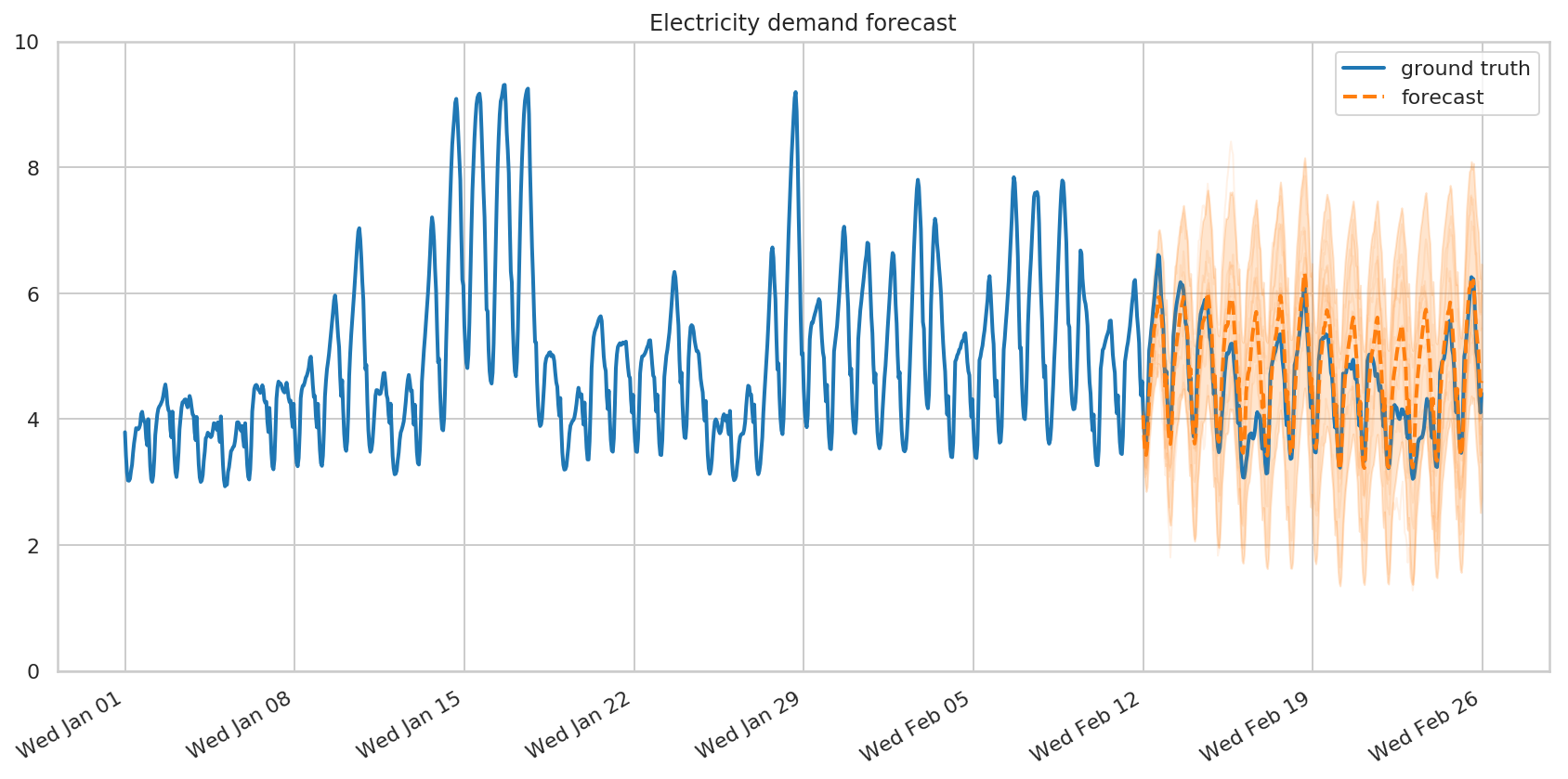
חיזוי וביקורת
שוב, אנו יוצרים תחזית פשוט על ידי קריאה ל- tfp.sts.forecast עם המודל שלנו, סדרת הזמן והפרמטרים שנדגמו.
demand_forecast_dist = tfp.sts.forecast(
    model=demand_model,
    observed_time_series=demand_training_data,
    parameter_samples=q_samples_demand_,
    num_steps_forecast=num_forecast_steps)
num_samples=10

(
    demand_forecast_mean,
    demand_forecast_scale,
    demand_forecast_samples
) = (
    demand_forecast_dist.mean().numpy()[..., 0],
    demand_forecast_dist.stddev().numpy()[..., 0],
    demand_forecast_dist.sample(num_samples).numpy()[..., 0]
    )
fig, ax = plot_forecast(demand_dates, demand,
                        demand_forecast_mean,
                        demand_forecast_scale,
                        demand_forecast_samples,
                        title="Electricity demand forecast",
                        x_locator=demand_loc, x_formatter=demand_fmt)
ax.set_ylim([0, 10])
fig.tight_layout()
בואו נדמיין את הפירוק של הסדרות הנצפות והחזויות לרכיבים בודדים:
# Get the distributions over component outputs from the posterior marginals on
# training data, and from the forecast model.
component_dists = sts.decompose_by_component(
    demand_model,
    observed_time_series=demand_training_data,
    parameter_samples=q_samples_demand_)

forecast_component_dists = sts.decompose_forecast_by_component(
    demand_model,
    forecast_dist=demand_forecast_dist,
    parameter_samples=q_samples_demand_)
demand_component_means_, demand_component_stddevs_ = (
    {k.name: c.mean() for k, c in component_dists.items()},
    {k.name: c.stddev() for k, c in component_dists.items()})

(
    demand_forecast_component_means_,
    demand_forecast_component_stddevs_
) = (
    {k.name: c.mean() for k, c in forecast_component_dists.items()},
    {k.name: c.stddev() for k, c in forecast_component_dists.items()}
    )
# Concatenate the training data with forecasts for plotting.
component_with_forecast_means_ = collections.OrderedDict()
component_with_forecast_stddevs_ = collections.OrderedDict()
for k in demand_component_means_.keys():
  component_with_forecast_means_[k] = np.concatenate([
      demand_component_means_[k],
      demand_forecast_component_means_[k]], axis=-1)
  component_with_forecast_stddevs_[k] = np.concatenate([
      demand_component_stddevs_[k],
      demand_forecast_component_stddevs_[k]], axis=-1)


fig, axes = plot_components(
  demand_dates,
  component_with_forecast_means_,
  component_with_forecast_stddevs_,
  x_locator=demand_loc, x_formatter=demand_fmt)
for ax in axes.values():
  ax.axvline(demand_dates[-num_forecast_steps], linestyle="--", color='red')

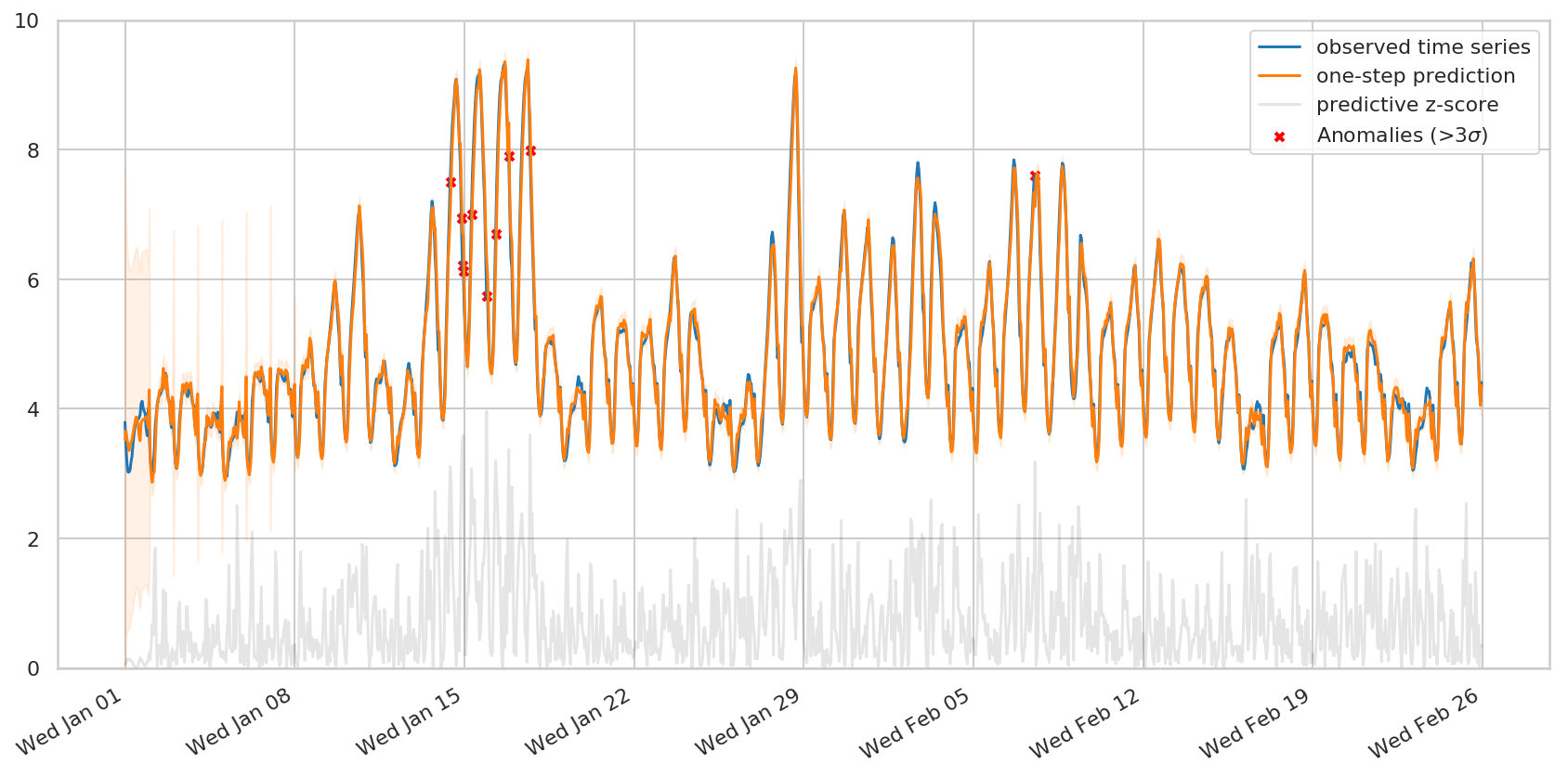
אם היינו רוצים לזהות חריגות בסדרה הנצפית, אולי נתעניין גם בהתפלגויות החזויות של שלב אחד: התחזית עבור כל שלב זמן, בהינתן רק שלבי הזמן עד לאותה נקודה. tfp.sts.one_step_predictive מחשב את כל ההפצות החזויות בשלב אחד במעבר אחד:
demand_one_step_dist = sts.one_step_predictive(
    demand_model,
    observed_time_series=demand,
    parameter_samples=q_samples_demand_)

demand_one_step_mean, demand_one_step_scale = (
    demand_one_step_dist.mean().numpy(), demand_one_step_dist.stddev().numpy())
תוכנית פשוטה לזיהוי חריגות היא לסמן את כל שלבי הזמן שבהם התצפיות הן יותר משלושה סטddevs מהערך החזוי -- אלו הם שלבי הזמן ה"מפתיעים" ביותר לפי המודל.
fig, ax = plot_one_step_predictive(
    demand_dates, demand,
    demand_one_step_mean, demand_one_step_scale,
    x_locator=demand_loc, x_formatter=demand_fmt)
ax.set_ylim(0, 10)

# Use the one-step-ahead forecasts to detect anomalous timesteps.
zscores = np.abs((demand - demand_one_step_mean) /
                 demand_one_step_scale)
anomalies = zscores > 3.0
ax.scatter(demand_dates[anomalies],
           demand[anomalies],
           c="red", marker="x", s=20, linewidth=2, label=r"Anomalies (>3$\sigma$)")
ax.plot(demand_dates, zscores, color="black", alpha=0.1, label='predictive z-score')
ax.legend()
plt.show()