TensorFlow 14 मई को Google I/O पर वापस आ गया है! अभी पंजीकरण करें

इस पेज का अनुवाद Cloud Translation API से किया गया है.

TFP रिलीज़ नोट्स नोटबुक (0.13.0)

इस नोटबुक का उद्देश्य कुछ छोटे स्निपेट्स के माध्यम से TFP 0.13.0 को "जीवन में आने" में मदद करना है - TFP के साथ आप जो चीजें हासिल कर सकते हैं, उनके छोटे डेमो।

TensorFlow.org पर देखें

Google Colab में चलाएं

GitHub पर स्रोत देखें

नोटबुक डाउनलोड करें

इंस्टॉल और आयात

!pip3 install -qU tensorflow==2.5.0 tensorflow_probability==0.13.0 tensorflow-datasets inference_gym

import tensorflow as tf
import tensorflow_probability as tfp
assert '0.13' in tfp.__version__, tfp.__version__
assert '2.5' in tf.__version__, tf.__version__

physical_devices = tf.config.list_physical_devices('CPU')
tf.config.set_logical_device_configuration(
    physical_devices[0],
    [tf.config.LogicalDeviceConfiguration(),
     tf.config.LogicalDeviceConfiguration()])

tfd = tfp.distributions
tfb = tfp.bijectors
tfpk = tfp.math.psd_kernels

import matplotlib.pyplot as plt
import numpy as np
import scipy.interpolate
import IPython
import seaborn as sns
import logging

[K     |████████████████████████████████| 5.4MB 8.8MB/s 
[K     |████████████████████████████████| 3.9MB 37.1MB/s 
[K     |████████████████████████████████| 296kB 31.6MB/s 
[?25h

वितरण [कोर गणित]

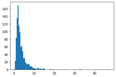
`BetaQuotient`

दो स्वतंत्र बीटा-वितरित यादृच्छिक चर का अनुपात

plt.hist(tfd.BetaQuotient(concentration1_numerator=5.,
                          concentration0_numerator=2.,
                          concentration1_denominator=3.,
                          concentration0_denominator=8.).sample(1_000, seed=(1, 23)),
         bins='auto');

पीएनजी

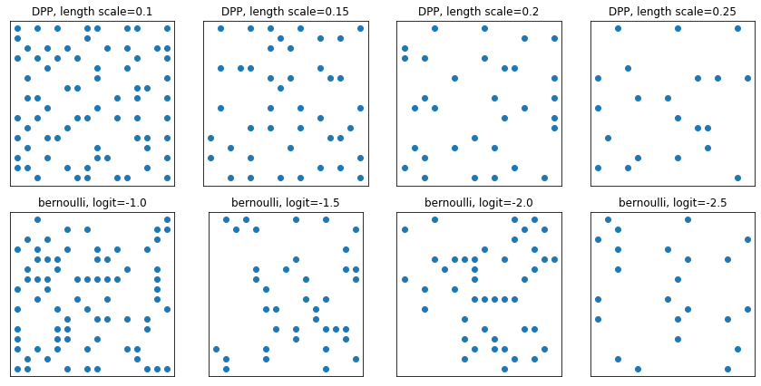
`DeterminantalPointProcess`

किसी दिए गए सेट के सबसेट (एक-हॉट के रूप में दर्शाया गया) पर वितरण। नमूने एक प्रतिकर्षण गुण का अनुसरण करते हैं (संभावनाएं बिंदुओं के चयनित उपसमुच्चय के अनुरूप वैक्टर द्वारा फैले आयतन के समानुपाती होती हैं), जो विविध उपसमुच्चय के नमूने की ओर जाता है। [आईआईडी बर्नौली नमूनों से तुलना करें।]

grid_size = 16
# Generate grid_size**2 pts on the unit square.
grid = np.arange(0, 1, 1./grid_size).astype(np.float32)
import itertools
points = np.array(list(itertools.product(grid, grid)))

# Create the kernel L that parameterizes the DPP.
kernel_amplitude = 2.
kernel_lengthscale = [.1, .15, .2, .25]  # Increasing length scale indicates more points are "nearby", tending toward smaller subsets.
kernel = tfpk.ExponentiatedQuadratic(kernel_amplitude, kernel_lengthscale)
kernel_matrix = kernel.matrix(points, points)

eigenvalues, eigenvectors = tf.linalg.eigh(kernel_matrix)
dpp = tfd.DeterminantalPointProcess(eigenvalues, eigenvectors)
print(dpp)

# The inner-most dimension of the result of `dpp.sample` is a multi-hot
# encoding of a subset of {1, ..., ground_set_size}.
# We will compare against a bernoulli distribution.
samps_dpp = dpp.sample(seed=(1, 2))  # 4 x grid_size**2
logits = tf.broadcast_to([[-1.], [-1.5], [-2], [-2.5]], [4, grid_size**2])
samps_bern = tfd.Bernoulli(logits=logits).sample(seed=(2, 3))

plt.figure(figsize=(12, 6))
for i, (samp, samp_bern) in enumerate(zip(samps_dpp, samps_bern)):
  plt.subplot(241 + i)
  plt.scatter(*points[np.where(samp)].T)
  plt.title(f'DPP, length scale={kernel_lengthscale[i]}')
  plt.xticks([])
  plt.yticks([])
  plt.gca().set_aspect(1.)
  plt.subplot(241 + i + 4)
  plt.scatter(*points[np.where(samp_bern)].T)
  plt.title(f'bernoulli, logit={logits[i,0]}')
  plt.xticks([])
  plt.yticks([])
  plt.gca().set_aspect(1.)

plt.tight_layout()
plt.show()

tfp.distributions.DeterminantalPointProcess("DeterminantalPointProcess", batch_shape=[4], event_shape=[256], dtype=int32)

पीएनजी

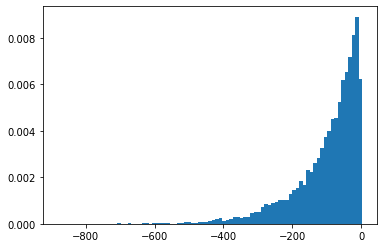
`SigmoidBeta`

दो गामा वितरणों के लॉग-ऑड्स। अधिक से अधिक संख्यानुसार स्थिर नमूना अंतरिक्ष Beta ।

plt.hist(tfd.SigmoidBeta(concentration1=.01, concentration0=2.).sample(10_000, seed=(1, 23)),
         bins='auto', density=True);
plt.show()

print('Old way, fractions non-finite:')
print(np.sum(~tf.math.is_finite(
    tfb.Invert(tfb.Sigmoid())(tfd.Beta(concentration1=.01, concentration0=2.)).sample(10_000, seed=(1, 23)))) / 10_000)
print(np.sum(~tf.math.is_finite(
    tfb.Invert(tfb.Sigmoid())(tfd.Beta(concentration1=2., concentration0=.01)).sample(10_000, seed=(2, 34)))) / 10_000)

पीएनजी

Old way, fractions non-finite:
0.4215
0.8624

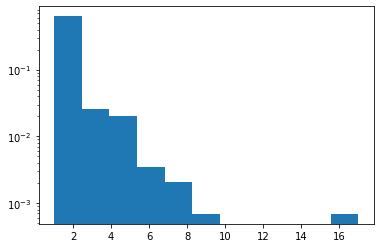
जिप्फ

JAX समर्थन जोड़ा गया।

plt.hist(tfd.Zipf(3.).sample(1_000, seed=(12, 34)).numpy(), bins='auto', density=True, log=True);

पीएनजी

`NormalInverseGaussian`

लचीला पैरामीट्रिक परिवार जो भारी पूंछ, तिरछी और वेनिला सामान्य का समर्थन करता है।

`MatrixNormalLinearOperator`

मैट्रिक्स सामान्य वितरण।

# Initialize a single 2 x 3 Matrix Normal.
mu = [[1., 2, 3], [3., 4, 5]]
col_cov = [[ 0.36,  0.12,  0.06],
           [ 0.12,  0.29, -0.13],
           [ 0.06, -0.13,  0.26]]
scale_column = tf.linalg.LinearOperatorLowerTriangular(tf.linalg.cholesky(col_cov))
scale_row = tf.linalg.LinearOperatorDiag([0.9, 0.8])

mvn = tfd.MatrixNormalLinearOperator(loc=mu, scale_row=scale_row, scale_column=scale_column)
mvn.sample()

WARNING:tensorflow:From /usr/local/lib/python3.7/dist-packages/tensorflow/python/ops/linalg/linear_operator_kronecker.py:224: LinearOperator.graph_parents (from tensorflow.python.ops.linalg.linear_operator) is deprecated and will be removed in a future version.
Instructions for updating:
Do not call `graph_parents`.
<tf.Tensor: shape=(2, 3), dtype=float32, numpy=
array([[1.2495145, 1.549366 , 3.2748342],
       [3.7330258, 4.3413105, 4.83423  ]], dtype=float32)>

`MatrixStudentTLinearOperator`

मैट्रिक्स टी वितरण।

mu = [[1., 2, 3], [3., 4, 5]]
col_cov = [[ 0.36,  0.12,  0.06],
           [ 0.12,  0.29, -0.13],
           [ 0.06, -0.13,  0.26]]
scale_column = tf.linalg.LinearOperatorLowerTriangular(tf.linalg.cholesky(col_cov))
scale_row = tf.linalg.LinearOperatorDiag([0.9, 0.8])

mvn = tfd.MatrixTLinearOperator(
    df=2.,
    loc=mu,
    scale_row=scale_row,
    scale_column=scale_column)
mvn.sample()

<tf.Tensor: shape=(2, 3), dtype=float32, numpy=
array([[1.6549466, 2.6708362, 2.8629923],
       [2.1222284, 3.6904747, 5.08014  ]], dtype=float32)>

वितरण [सॉफ्टवेयर / रैपर]

`Sharded`

एकाधिक प्रोसेसरों में वितरण के स्वतंत्र ईवेंट भाग को शार्प करता है। समुच्चय log_prob के साथ मिलकर सभी डिवाइस में, हैंडल ढ़ाल tfp.experimental.distribute.JointDistribution* । ज्यादातर में और अधिक वितरित निष्कर्ष नोटबुक।

strategy = tf.distribute.MirroredStrategy()

@tf.function
def sample_and_lp(seed):
  d = tfp.experimental.distribute.Sharded(tfd.Normal(0, 1))
  s = d.sample(seed=seed)
  return s, d.log_prob(s)

strategy.run(sample_and_lp, args=(tf.constant([12,34]),))

WARNING:tensorflow:There are non-GPU devices in `tf.distribute.Strategy`, not using nccl allreduce.
WARNING:tensorflow:Collective ops is not configured at program startup. Some performance features may not be enabled.
INFO:tensorflow:Using MirroredStrategy with devices ('/job:localhost/replica:0/task:0/device:CPU:0', '/job:localhost/replica:0/task:0/device:CPU:1')
INFO:tensorflow:Reduce to /job:localhost/replica:0/task:0/device:CPU:0 then broadcast to ('/job:localhost/replica:0/task:0/device:CPU:0', '/job:localhost/replica:0/task:0/device:CPU:1').
(PerReplica:{
   0: <tf.Tensor: shape=(), dtype=float32, numpy=0.0051413667>,
   1: <tf.Tensor: shape=(), dtype=float32, numpy=-0.3393052>
 }, PerReplica:{
   0: <tf.Tensor: shape=(), dtype=float32, numpy=-1.8954543>,
   1: <tf.Tensor: shape=(), dtype=float32, numpy=-1.8954543>
 })

`BatchBroadcast`

परोक्ष साथ या किसी दिए गए बैच आकार के एक अंतर्निहित वितरण के बैच आयाम प्रसारण करते हैं।

underlying = tfd.MultivariateNormalDiag(tf.zeros([7, 1, 5]), tf.ones([5]))
print('underlying:', underlying)

d = tfd.BatchBroadcast(underlying, [8, 1, 6])
print('broadcast [7, 1] *with* [8, 1, 6]:', d)

try:
  tfd.BatchBroadcast(underlying, to_shape=[8, 1, 6])
except ValueError as e:
  print('broadcast [7, 1] *to* [8, 1, 6] is invalid:', e)

d = tfd.BatchBroadcast(underlying, to_shape=[8, 7, 6])
print('broadcast [7, 1] *to* [8, 7, 6]:', d)

underlying: tfp.distributions.MultivariateNormalDiag("MultivariateNormalDiag", batch_shape=[7, 1], event_shape=[5], dtype=float32)
broadcast [7, 1] *with* [8, 1, 6]: tfp.distributions.BatchBroadcast("BatchBroadcastMultivariateNormalDiag", batch_shape=[8, 7, 6], event_shape=[5], dtype=float32)
broadcast [7, 1] *to* [8, 1, 6] is invalid: Argument `to_shape` ([8 1 6]) is incompatible with underlying distribution batch shape ((7, 1)).
broadcast [7, 1] *to* [8, 7, 6]: tfp.distributions.BatchBroadcast("BatchBroadcastMultivariateNormalDiag", batch_shape=[8, 7, 6], event_shape=[5], dtype=float32)

`Masked`

एकल कार्यक्रम / बहु-डेटा या विरल के रूप में नकाबपोश सघन उपयोग-मामले, एक वितरण के लिए है कि बाहर मास्क log_prob अमान्य अंतर्निहित वितरण का।

d = tfd.Masked(tfd.Normal(tf.zeros([7]), 1), 
               validity_mask=tf.sequence_mask([3, 4], 7))
print(d.log_prob(d.sample(seed=(1, 1))))

d = tfd.Masked(tfd.Normal(0, 1), 
               validity_mask=[False, True, False],
               safe_sample_fn=tfd.Distribution.mode)
print(d.log_prob(d.sample(seed=(2, 2))))

tf.Tensor(
[[-2.3054113 -1.8524303 -1.2220721  0.         0.         0.

   0.       ]
 [-1.118623  -1.1370811 -1.1574132 -5.884986   0.         0.
   0.       ]], shape=(2, 7), dtype=float32)
tf.Tensor([ 0.         -0.93683904  0.        ], shape=(3,), dtype=float32)

बिजेक्टर

बिजेक्टर
- नकल करने के लिए bijectors जोड़े tf.nest.flatten ( tfb.tree_flatten ) और tf.nest.pack_sequence_as ( tfb.pack_sequence_as )।
- जोड़ता tfp.experimental.bijectors.Sharded
- निकालें पदावनत tfb.ScaleTrilL । उपयोग tfb.FillScaleTriL बजाय।
- जोड़ता है cls.parameter_properties() Bijectors के लिए एनोटेशन।
- सीमा का विस्तार tfb.Power विषम पूर्णांक शक्तियों के लिए सभी reals करने के लिए।
- यदि अन्यथा निर्दिष्ट नहीं है, तो ऑटोडिफ का उपयोग करके स्केलर बायजेक्टर के लॉग-डिग-जैकोबियन का अनुमान लगाएं।

पुनर्रचना बायजेक्टर

ex = (tf.constant(1.), dict(b=tf.constant(2.), c=tf.constant(3.)))
b = tfb.tree_flatten(ex)
print(b.forward(ex))
print(b.inverse(list(tf.constant([1., 2, 3]))))

b = tfb.pack_sequence_as(ex)
print(b.forward(list(tf.constant([1., 2, 3]))))
print(b.inverse(ex))

[<tf.Tensor: shape=(), dtype=float32, numpy=1.0>, <tf.Tensor: shape=(), dtype=float32, numpy=2.0>, <tf.Tensor: shape=(), dtype=float32, numpy=3.0>]
(<tf.Tensor: shape=(), dtype=float32, numpy=1.0>, {'b': <tf.Tensor: shape=(), dtype=float32, numpy=2.0>, 'c': <tf.Tensor: shape=(), dtype=float32, numpy=3.0>})
(<tf.Tensor: shape=(), dtype=float32, numpy=1.0>, {'b': <tf.Tensor: shape=(), dtype=float32, numpy=2.0>, 'c': <tf.Tensor: shape=(), dtype=float32, numpy=3.0>})
[<tf.Tensor: shape=(), dtype=float32, numpy=1.0>, <tf.Tensor: shape=(), dtype=float32, numpy=2.0>, <tf.Tensor: shape=(), dtype=float32, numpy=3.0>]

`Sharded`

लॉग-निर्धारक में एसपीएमडी कमी। देखें Sharded नीचे वितरण में,।

strategy = tf.distribute.MirroredStrategy()

def sample_lp_logdet(seed):
  d = tfd.TransformedDistribution(tfp.experimental.distribute.Sharded(tfd.Normal(0, 1), shard_axis_name='i'),
                                  tfp.experimental.bijectors.Sharded(tfb.Sigmoid(), shard_axis_name='i'))
  s = d.sample(seed=seed)
  return s, d.log_prob(s), d.bijector.inverse_log_det_jacobian(s)
strategy.run(sample_lp_logdet, (tf.constant([1, 2]),))

WARNING:tensorflow:There are non-GPU devices in `tf.distribute.Strategy`, not using nccl allreduce.
WARNING:tensorflow:Collective ops is not configured at program startup. Some performance features may not be enabled.
INFO:tensorflow:Using MirroredStrategy with devices ('/job:localhost/replica:0/task:0/device:CPU:0', '/job:localhost/replica:0/task:0/device:CPU:1')
WARNING:tensorflow:Using MirroredStrategy eagerly has significant overhead currently. We will be working on improving this in the future, but for now please wrap `call_for_each_replica` or `experimental_run` or `run` inside a tf.function to get the best performance.
INFO:tensorflow:Reduce to /job:localhost/replica:0/task:0/device:CPU:0 then broadcast to ('/job:localhost/replica:0/task:0/device:CPU:0', '/job:localhost/replica:0/task:0/device:CPU:1').
INFO:tensorflow:Reduce to /job:localhost/replica:0/task:0/device:CPU:0 then broadcast to ('/job:localhost/replica:0/task:0/device:CPU:0', '/job:localhost/replica:0/task:0/device:CPU:1').
(PerReplica:{
   0: <tf.Tensor: shape=(), dtype=float32, numpy=0.87746525>,
   1: <tf.Tensor: shape=(), dtype=float32, numpy=0.24580425>
 }, PerReplica:{
   0: <tf.Tensor: shape=(), dtype=float32, numpy=-0.48870325>,
   1: <tf.Tensor: shape=(), dtype=float32, numpy=-0.48870325>
 }, PerReplica:{
   0: <tf.Tensor: shape=(), dtype=float32, numpy=3.9154015>,
   1: <tf.Tensor: shape=(), dtype=float32, numpy=3.9154015>
 })

छठी

जोड़ता build_split_flow_surrogate_posterior को tfp.experimental.vi छठी किराए की कूल्हे संरचित निर्माण करने के लिए सामान्य से बहती से।
जोड़ता build_affine_surrogate_posterior को tfp.experimental.vi एक घटना आकृति से advi किराए की कूल्हे के निर्माण के लिए।
जोड़ता build_affine_surrogate_posterior_from_base_distribution को tfp.experimental.vi परिवर्तनों affine से प्रेरित सहसंबंध संरचनाओं के साथ advi किराए की कूल्हे के निर्माण कर सकें।

VI/एमएपी/एमएलई

अतिरिक्त सुविधा विधि tfp.experimental.util.make_trainable(cls) वितरण और bijectors की trainable उदाहरणों बनाने के लिए।

d = tfp.experimental.util.make_trainable(tfd.Gamma)
print(d.trainable_variables)
print(d)

(<tf.Variable 'Gamma_trainable_variables/concentration:0' shape=() dtype=float32, numpy=1.0296053>, <tf.Variable 'Gamma_trainable_variables/log_rate:0' shape=() dtype=float32, numpy=-0.3465951>)
tfp.distributions.Gamma("Gamma", batch_shape=[], event_shape=[], dtype=float32)

एमसीएमसी

एमसीएमसी डायग्नोस्टिक्स सिर्फ सूचियां ही नहीं, बल्कि राज्यों के मनमाने ढांचे का समर्थन करते हैं।
remc_thermodynamic_integrals को जोड़ा गया tfp.experimental.mcmc
जोड़ता tfp.experimental.mcmc.windowed_adaptive_hmc
अप्रतिबंधित स्थान में लगभग-शून्य समान वितरण से मार्कोव श्रृंखला को प्रारंभ करने के लिए एक प्रयोगात्मक एपीआई जोड़ता है। tfp.experimental.mcmc.init_near_unconstrained_zero
एक स्वीकार्य बिंदु मिलने तक मार्कोव चेन इनिशियलाइज़ेशन को पुनः प्रयास करने के लिए एक प्रयोगात्मक उपयोगिता जोड़ता है। tfp.experimental.mcmc.retry_init
कम से कम व्यवधान के साथ tfp.mcmc में स्लॉट करने के लिए प्रयोगात्मक स्ट्रीमिंग MCMC API को शफ़ल करना।
जोड़ता ThinningKernel को experimental.mcmc ।
जोड़ता experimental.mcmc.run_kernel एक उम्मीदवार के रूप चालक स्ट्रीमिंग-आधारित करने के लिए प्रतिस्थापन mcmc.sample_chain

`init_near_unconstrained_zero` , `retry_init`

@tfd.JointDistributionCoroutine
def model():
  Root = tfd.JointDistributionCoroutine.Root
  c0 = yield Root(tfd.Gamma(2, 2, name='c0'))
  c1 = yield Root(tfd.Gamma(2, 2, name='c1'))
  counts = yield tfd.Sample(tfd.BetaBinomial(23, c1, c0), 10, name='counts')
jd = model.experimental_pin(counts=model.sample(seed=[20, 30]).counts)

init_dist = tfp.experimental.mcmc.init_near_unconstrained_zero(jd)
print(init_dist)

tfp.experimental.mcmc.retry_init(init_dist.sample, jd.unnormalized_log_prob)

tfp.distributions.TransformedDistribution("default_joint_bijectorrestructureJointDistributionSequential", batch_shape=StructTuple(
  c0=[],
  c1=[]
), event_shape=StructTuple(
  c0=[],
  c1=[]
), dtype=StructTuple(
  c0=float32,
  c1=float32
))
StructTuple(
  c0=<tf.Tensor: shape=(), dtype=float32, numpy=1.7879653>,
  c1=<tf.Tensor: shape=(), dtype=float32, numpy=0.34548905>
)

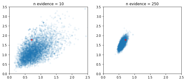
विंडो अनुकूली एचएमसी और एनयूटीएस नमूने

fig, ax = plt.subplots(1, 2, figsize=(10, 4))
for i, n_evidence in enumerate((10, 250)):
  ax[i].set_title(f'n evidence = {n_evidence}')
  ax[i].set_xlim(0, 2.5); ax[i].set_ylim(0, 3.5)
  @tfd.JointDistributionCoroutine
  def model():
    Root = tfd.JointDistributionCoroutine.Root
    c0 = yield Root(tfd.Gamma(2, 2, name='c0'))
    c1 = yield Root(tfd.Gamma(2, 2, name='c1'))
    counts = yield tfd.Sample(tfd.BetaBinomial(23, c1, c0), n_evidence, name='counts')
  s = model.sample(seed=[20, 30])
  print(s)
  jd = model.experimental_pin(counts=s.counts)
  states, trace = tf.function(tfp.experimental.mcmc.windowed_adaptive_hmc)(
      100, jd, num_leapfrog_steps=5, seed=[100, 200])
  ax[i].scatter(states.c0.numpy().reshape(-1), states.c1.numpy().reshape(-1), 
                marker='+', alpha=.1)
  ax[i].scatter(s.c0, s.c1, marker='+', color='r')

StructTuple(
  c0=<tf.Tensor: shape=(), dtype=float32, numpy=0.7161876>,
  c1=<tf.Tensor: shape=(), dtype=float32, numpy=1.7696666>,
  counts=<tf.Tensor: shape=(10,), dtype=float32, numpy=array([ 6., 10., 23.,  7.,  2., 20., 14., 16., 22., 17.], dtype=float32)>
)
WARNING:tensorflow:6 out of the last 6 calls to <function windowed_adaptive_hmc at 0x7fda42bed8c0> triggered tf.function retracing. Tracing is expensive and the excessive number of tracings could be due to (1) creating @tf.function repeatedly in a loop, (2) passing tensors with different shapes, (3) passing Python objects instead of tensors. For (1), please define your @tf.function outside of the loop. For (2), @tf.function has experimental_relax_shapes=True option that relaxes argument shapes that can avoid unnecessary retracing. For (3), please refer to https://www.tensorflow.org/guide/function#controlling_retracing and https://www.tensorflow.org/api_docs/python/tf/function for  more details.
StructTuple(
  c0=<tf.Tensor: shape=(), dtype=float32, numpy=0.7161876>,
  c1=<tf.Tensor: shape=(), dtype=float32, numpy=1.7696666>,
  counts=<tf.Tensor: shape=(250,), dtype=float32, numpy=
    array([ 6., 10., 23.,  7.,  2., 20., 14., 16., 22., 17., 22., 21.,  6.,
           21., 12., 22., 23., 16., 18., 21., 16., 17., 17., 16., 21., 14.,
           23., 15., 10., 19.,  8., 23., 23., 14.,  1., 23., 16., 22., 20.,
           20., 22., 15., 16., 20., 20., 21., 23., 22., 21., 15., 18., 23.,
           12., 16., 19., 23., 18.,  5., 22., 22., 22., 18., 12., 17., 17.,
           16.,  8., 22., 20., 23.,  3., 12., 14., 18.,  7., 19., 19.,  9.,
           10., 23., 14., 22., 22., 21., 13., 23., 14., 23., 10., 17., 23.,
           17., 20., 16., 20., 19., 14.,  0., 17., 22., 12.,  2., 17., 15.,
           14., 23., 19., 15., 23.,  2., 21., 23., 21.,  7., 21., 12., 23.,
           17., 17.,  4., 22., 16., 14., 19., 19., 20.,  6., 16., 14., 18.,
           21., 12., 21., 21., 22.,  2., 19., 11.,  6., 19.,  1., 23., 23.,
           14.,  6., 23., 18.,  8., 20., 23., 13., 20., 18., 23., 17., 22.,
           23., 20., 18., 22., 16., 23.,  9., 22., 21., 16., 20., 21., 16.,
           23.,  7., 13., 23., 19.,  3., 13., 23., 23., 13., 19., 23., 20.,
           18.,  8., 19., 14., 12.,  6.,  8., 23.,  3., 13., 21., 23., 22.,
           23., 19., 22., 21., 15., 22., 21., 21., 23.,  9., 19., 20., 23.,
           11., 23., 14., 23., 14., 21., 21., 10., 23.,  9., 13.,  1.,  8.,
            8., 20., 21., 21., 21., 14., 16., 16.,  9., 23., 22., 11., 23.,
           12., 18.,  1., 23.,  9.,  3., 21., 21., 23., 22., 18., 23., 16.,
            3., 11., 16.], dtype=float32)>
)

पीएनजी

गणित, आँकड़े

गणित/लिनालग
- जोड़े tfp.math.trapz समलम्बाकार एकीकरण के लिए।
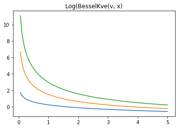
- जोड़े tfp.math.log_bessel_kve ।
- जोड़े no_pivot_ldl को experimental.linalg ।
- जोड़े marginal_fn को तर्क GaussianProcess (देखें no_pivot_ldl )।
- जोड़ा tfp.math.atan_difference(x, y)
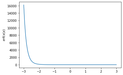
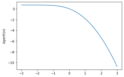
- जोड़े tfp.math.erfcx , tfp.math.logerfc और tfp.math.logerfcx
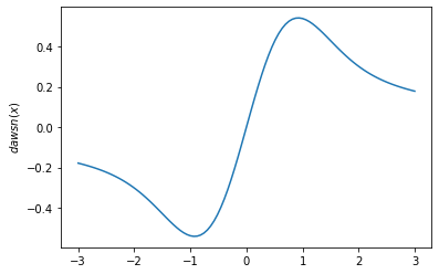
- जोड़े tfp.math.dawsn डावसन इंटीग्रल के लिए।
- जोड़े tfp.math.igammaincinv , tfp.math.igammacinv ।
- जोड़े tfp.math.sqrt1pm1 ।
- जोड़े LogitNormal.stddev_approx और LogitNormal.variance_approx
- जोड़े tfp.math.owens_t ओवेन के टी समारोह के लिए।
- जोड़े bracket_root एक रूट खोज के लिए स्वचालित रूप से इनिशियलाइज़ सीमा को विधि।
- अदिश फलनों के मूल ज्ञात करने के लिए चंद्रपतला की विधि जोड़ें।
आँकड़े
- tfp.stats.windowed_mean कुशलतापूर्वक विंडोड गणना करता है इसका मतलब है।
- tfp.stats.windowed_variance कुशलता से और सही ढंग से computes विडों प्रसरण।
- tfp.stats.cumulative_variance कुशलता से और सही ढंग से संचयी प्रसरण की गणना करता है।
- RunningCovariance और दोस्तों अब, एक उदाहरण टेन्सर से प्रारंभ किया जा सकता है न सिर्फ स्पष्ट आकार और dtype से।
- के लिए क्लीनर एपीआई RunningCentralMoments , RunningMean , RunningPotentialScaleReduction ।

ओवेन्स टी, एरफक्स, लॉगरफक, लॉगरफक्स, डावसन फंक्शन

# Owen's T gives the probability that X > h, 0 < Y < a * X. Let's check that
# with random sampling.
h = np.array([1., 2.]).astype(np.float32)
a = np.array([10., 11.5]).astype(np.float32)
probs = tfp.math.owens_t(h, a)

x = tfd.Normal(0., 1.).sample(int(1e5), seed=(6, 245)).numpy()
y = tfd.Normal(0., 1.).sample(int(1e5), seed=(7, 245)).numpy()

true_values = (
    (x[..., np.newaxis] > h) &
    (0. < y[..., np.newaxis]) &
    (y[..., np.newaxis] < a * x[..., np.newaxis]))

print('Calculated values: {}'.format(
    np.count_nonzero(true_values, axis=0) / 1e5))

print('Expected values: {}'.format(probs))

Calculated values: [0.07896 0.01134]
Expected values: [0.07932763 0.01137507]

x = np.linspace(-3., 3., 100)
plt.plot(x, tfp.math.erfcx(x))
plt.ylabel('$erfcx(x)$')
plt.show()

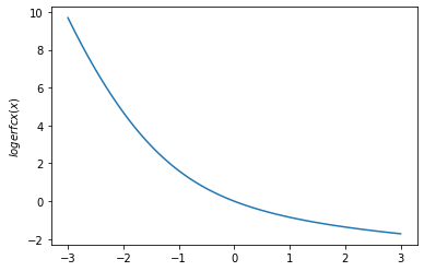
plt.plot(x, tfp.math.logerfcx(x))
plt.ylabel('$logerfcx(x)$')
plt.show()

plt.plot(x, tfp.math.logerfc(x))
plt.ylabel('$logerfc(x)$')
plt.show()

plt.plot(x, tfp.math.dawsn(x))
plt.ylabel('$dawsn(x)$')
plt.show()

पीएनजी

इगममैनव / इगम्मासिन्व

# Igammainv and Igammacinv are inverses to Igamma and Igammac

x = np.linspace(1., 10., 10)
y = tf.math.igamma(0.3, x)
x_prime = tfp.math.igammainv(0.3, y)
print('x: {}'.format(x))
print('igammainv(igamma(a, x)):\n {}'.format(x_prime))

y = tf.math.igammac(0.3, x)
x_prime = tfp.math.igammacinv(0.3, y)

print('\n')
print('x: {}'.format(x))
print('igammacinv(igammac(a, x)):\n {}'.format(x_prime))

x: [ 1.  2.  3.  4.  5.  6.  7.  8.  9. 10.]
igammainv(igamma(a, x)):
 [1.        1.9999992 3.000003  4.0000024 5.0000257 5.999887  7.0002484
 7.999243  8.99872   9.994673 ]


x: [ 1.  2.  3.  4.  5.  6.  7.  8.  9. 10.]
igammacinv(igammac(a, x)):
 [1.       2.       3.       4.       5.       6.       7.       8.000001

 9.       9.999999]

लॉग-केवीई

x = np.linspace(0., 5., 100)
for v in [0.5, 2., 3]:
  plt.plot(x, tfp.math.log_bessel_kve(v, x).numpy())

plt.title('Log(BesselKve(v, x)')

Text(0.5, 1.0, 'Log(BesselKve(v, x)')

पीएनजी

अन्य

अनुसूचित जनजातियों
- एसटीएस पूर्वानुमान और अपघटन आंतरिक का उपयोग कर में तेजी लाने के tf.function रैपिंग।
- विकल्प में छानने में तेजी लाने में जोड़े LinearGaussianSSM जब केवल अंतिम चरण के परिणाम की आवश्यकता है।
- संयुक्त वितरण के साथ परिवर्तन संबंधी निष्कर्ष: रेडॉन मॉडल के साथ उदाहरण नोटबुक ।
- किसी भी वितरण को प्रीकंडीशनिंग बायजेक्टर में बदलने के लिए प्रयोगात्मक समर्थन जोड़ें।
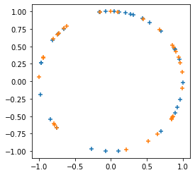
जोड़ता tfp.random.sanitize_seed ।
जोड़ता tfp.random.spherical_uniform ।

plt.figure(figsize=(4, 4))
seed = tfp.random.sanitize_seed(123)
seed1, seed2 = tfp.random.split_seed(seed)
samps = tfp.random.spherical_uniform([30], dimension=2, seed=seed1)
plt.scatter(*samps.numpy().T, marker='+')
samps = tfp.random.spherical_uniform([30], dimension=2, seed=seed2)
plt.scatter(*samps.numpy().T, marker='+');

पीएनजी

TFP रिलीज़ नोट्स नोटबुक (0.13.0)

इंस्टॉल और आयात

वितरण [कोर गणित]

BetaQuotient

DeterminantalPointProcess

SigmoidBeta

जिप्फ

NormalInverseGaussian

MatrixNormalLinearOperator

MatrixStudentTLinearOperator

वितरण [सॉफ्टवेयर / रैपर]

Sharded

BatchBroadcast

Masked

बिजेक्टर

पुनर्रचना बायजेक्टर

Sharded

छठी

VI/एमएपी/एमएलई

एमसीएमसी

init_near_unconstrained_zero , retry_init

विंडो अनुकूली एचएमसी और एनयूटीएस नमूने

गणित, आँकड़े

ओवेन्स टी, एरफक्स, लॉगरफक, लॉगरफक्स, डावसन फंक्शन

इगममैनव / इगम्मासिन्व

लॉग-केवीई

अन्य

`BetaQuotient`

`DeterminantalPointProcess`

`SigmoidBeta`

`NormalInverseGaussian`

`MatrixNormalLinearOperator`

`MatrixStudentTLinearOperator`

`Sharded`

`BatchBroadcast`

`Masked`

`Sharded`

`init_near_unconstrained_zero` , `retry_init`