Trang này được dịch bởi Cloud Translation API.

Sổ ghi chú phát hành TFP (0.13.0)

Mục đích của máy tính xách tay này là giúp TFP 0.13.0 "trở nên sống động" thông qua một số đoạn trích nhỏ - bản trình diễn nhỏ về những điều bạn có thể đạt được với TFP.

Xem trên TensorFlow.org

Chạy trong Google Colab

Xem nguồn trên GitHub

Tải xuống sổ ghi chép

Cài đặt và nhập

!pip3 install -qU tensorflow==2.5.0 tensorflow_probability==0.13.0 tensorflow-datasets inference_gym

import tensorflow as tf
import tensorflow_probability as tfp
assert '0.13' in tfp.__version__, tfp.__version__
assert '2.5' in tf.__version__, tf.__version__

physical_devices = tf.config.list_physical_devices('CPU')
tf.config.set_logical_device_configuration(
    physical_devices[0],
    [tf.config.LogicalDeviceConfiguration(),
     tf.config.LogicalDeviceConfiguration()])

tfd = tfp.distributions
tfb = tfp.bijectors
tfpk = tfp.math.psd_kernels

import matplotlib.pyplot as plt
import numpy as np
import scipy.interpolate
import IPython
import seaborn as sns
import logging

[K     |████████████████████████████████| 5.4MB 8.8MB/s 
[K     |████████████████████████████████| 3.9MB 37.1MB/s 
[K     |████████████████████████████████| 296kB 31.6MB/s 
[?25h

Phân phối [toán học cốt lõi]

`BetaQuotient`

Tỷ lệ của hai biến ngẫu nhiên có phân phối Beta độc lập

plt.hist(tfd.BetaQuotient(concentration1_numerator=5.,
                          concentration0_numerator=2.,
                          concentration1_denominator=3.,
                          concentration0_denominator=8.).sample(1_000, seed=(1, 23)),
         bins='auto');

png

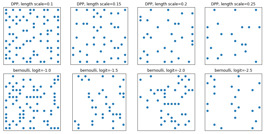
`DeterminantalPointProcess`

Phân phối trên các tập hợp con (được biểu diễn dưới dạng một nóng) của một tập hợp nhất định. Các mẫu tuân theo thuộc tính tính đẩy lùi (xác suất tỷ lệ với khối lượng được bao quanh bởi các vectơ tương ứng với tập con điểm đã chọn), có xu hướng lấy mẫu các tập con đa dạng. [So sánh với các mẫu Bernoulli iid.]

grid_size = 16
# Generate grid_size**2 pts on the unit square.
grid = np.arange(0, 1, 1./grid_size).astype(np.float32)
import itertools
points = np.array(list(itertools.product(grid, grid)))

# Create the kernel L that parameterizes the DPP.
kernel_amplitude = 2.
kernel_lengthscale = [.1, .15, .2, .25]  # Increasing length scale indicates more points are "nearby", tending toward smaller subsets.
kernel = tfpk.ExponentiatedQuadratic(kernel_amplitude, kernel_lengthscale)
kernel_matrix = kernel.matrix(points, points)

eigenvalues, eigenvectors = tf.linalg.eigh(kernel_matrix)
dpp = tfd.DeterminantalPointProcess(eigenvalues, eigenvectors)
print(dpp)

# The inner-most dimension of the result of `dpp.sample` is a multi-hot
# encoding of a subset of {1, ..., ground_set_size}.
# We will compare against a bernoulli distribution.
samps_dpp = dpp.sample(seed=(1, 2))  # 4 x grid_size**2
logits = tf.broadcast_to([[-1.], [-1.5], [-2], [-2.5]], [4, grid_size**2])
samps_bern = tfd.Bernoulli(logits=logits).sample(seed=(2, 3))

plt.figure(figsize=(12, 6))
for i, (samp, samp_bern) in enumerate(zip(samps_dpp, samps_bern)):
  plt.subplot(241 + i)
  plt.scatter(*points[np.where(samp)].T)
  plt.title(f'DPP, length scale={kernel_lengthscale[i]}')
  plt.xticks([])
  plt.yticks([])
  plt.gca().set_aspect(1.)
  plt.subplot(241 + i + 4)
  plt.scatter(*points[np.where(samp_bern)].T)
  plt.title(f'bernoulli, logit={logits[i,0]}')
  plt.xticks([])
  plt.yticks([])
  plt.gca().set_aspect(1.)

plt.tight_layout()
plt.show()

tfp.distributions.DeterminantalPointProcess("DeterminantalPointProcess", batch_shape=[4], event_shape=[256], dtype=int32)

png

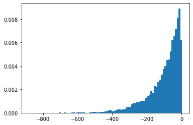
`SigmoidBeta`

Tỷ lệ đăng nhập của hai phân phối gamma. Số lượng nhiều không gian mẫu ổn định hơn Beta .

plt.hist(tfd.SigmoidBeta(concentration1=.01, concentration0=2.).sample(10_000, seed=(1, 23)),
         bins='auto', density=True);
plt.show()

print('Old way, fractions non-finite:')
print(np.sum(~tf.math.is_finite(
    tfb.Invert(tfb.Sigmoid())(tfd.Beta(concentration1=.01, concentration0=2.)).sample(10_000, seed=(1, 23)))) / 10_000)
print(np.sum(~tf.math.is_finite(
    tfb.Invert(tfb.Sigmoid())(tfd.Beta(concentration1=2., concentration0=.01)).sample(10_000, seed=(2, 34)))) / 10_000)

png

Old way, fractions non-finite:
0.4215
0.8624

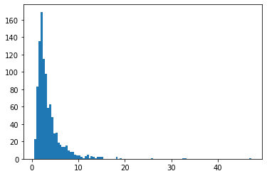
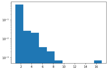
Zipf

Đã thêm hỗ trợ JAX.

plt.hist(tfd.Zipf(3.).sample(1_000, seed=(12, 34)).numpy(), bins='auto', density=True, log=True);

png

`NormalInverseGaussian`

Họ tham số linh hoạt hỗ trợ đuôi nặng, lệch và vani Bình thường.

`MatrixNormalLinearOperator`

Ma trận Phân phối chuẩn.

# Initialize a single 2 x 3 Matrix Normal.
mu = [[1., 2, 3], [3., 4, 5]]
col_cov = [[ 0.36,  0.12,  0.06],
           [ 0.12,  0.29, -0.13],
           [ 0.06, -0.13,  0.26]]
scale_column = tf.linalg.LinearOperatorLowerTriangular(tf.linalg.cholesky(col_cov))
scale_row = tf.linalg.LinearOperatorDiag([0.9, 0.8])

mvn = tfd.MatrixNormalLinearOperator(loc=mu, scale_row=scale_row, scale_column=scale_column)
mvn.sample()

WARNING:tensorflow:From /usr/local/lib/python3.7/dist-packages/tensorflow/python/ops/linalg/linear_operator_kronecker.py:224: LinearOperator.graph_parents (from tensorflow.python.ops.linalg.linear_operator) is deprecated and will be removed in a future version.
Instructions for updating:
Do not call `graph_parents`.
<tf.Tensor: shape=(2, 3), dtype=float32, numpy=
array([[1.2495145, 1.549366 , 3.2748342],
       [3.7330258, 4.3413105, 4.83423  ]], dtype=float32)>

`MatrixStudentTLinearOperator`

Ma trận T phân phối.

mu = [[1., 2, 3], [3., 4, 5]]
col_cov = [[ 0.36,  0.12,  0.06],
           [ 0.12,  0.29, -0.13],
           [ 0.06, -0.13,  0.26]]
scale_column = tf.linalg.LinearOperatorLowerTriangular(tf.linalg.cholesky(col_cov))
scale_row = tf.linalg.LinearOperatorDiag([0.9, 0.8])

mvn = tfd.MatrixTLinearOperator(
    df=2.,
    loc=mu,
    scale_row=scale_row,
    scale_column=scale_column)
mvn.sample()

<tf.Tensor: shape=(2, 3), dtype=float32, numpy=
array([[1.6549466, 2.6708362, 2.8629923],
       [2.1222284, 3.6904747, 5.08014  ]], dtype=float32)>

Phân phối [phần mềm / wrappers]

`Sharded`

Chia nhỏ các phần sự kiện độc lập của một bản phân phối trên nhiều bộ xử lý. Uẩn log_prob giữa các thiết bị, xử lý gradient phối hợp với tfp.experimental.distribute.JointDistribution* . Nhiều hơn nữa trong suy luận Distributed máy tính xách tay.

strategy = tf.distribute.MirroredStrategy()

@tf.function
def sample_and_lp(seed):
  d = tfp.experimental.distribute.Sharded(tfd.Normal(0, 1))
  s = d.sample(seed=seed)
  return s, d.log_prob(s)

strategy.run(sample_and_lp, args=(tf.constant([12,34]),))

WARNING:tensorflow:There are non-GPU devices in `tf.distribute.Strategy`, not using nccl allreduce.
WARNING:tensorflow:Collective ops is not configured at program startup. Some performance features may not be enabled.
INFO:tensorflow:Using MirroredStrategy with devices ('/job:localhost/replica:0/task:0/device:CPU:0', '/job:localhost/replica:0/task:0/device:CPU:1')
INFO:tensorflow:Reduce to /job:localhost/replica:0/task:0/device:CPU:0 then broadcast to ('/job:localhost/replica:0/task:0/device:CPU:0', '/job:localhost/replica:0/task:0/device:CPU:1').
(PerReplica:{
   0: <tf.Tensor: shape=(), dtype=float32, numpy=0.0051413667>,
   1: <tf.Tensor: shape=(), dtype=float32, numpy=-0.3393052>
 }, PerReplica:{
   0: <tf.Tensor: shape=(), dtype=float32, numpy=-1.8954543>,
   1: <tf.Tensor: shape=(), dtype=float32, numpy=-1.8954543>
 })

`BatchBroadcast`

Ngầm phát sóng kích thước hàng loạt của một phân phối tiềm ẩn với hoặc một hình dạng batch nhất định.

underlying = tfd.MultivariateNormalDiag(tf.zeros([7, 1, 5]), tf.ones([5]))
print('underlying:', underlying)

d = tfd.BatchBroadcast(underlying, [8, 1, 6])
print('broadcast [7, 1] *with* [8, 1, 6]:', d)

try:
  tfd.BatchBroadcast(underlying, to_shape=[8, 1, 6])
except ValueError as e:
  print('broadcast [7, 1] *to* [8, 1, 6] is invalid:', e)

d = tfd.BatchBroadcast(underlying, to_shape=[8, 7, 6])
print('broadcast [7, 1] *to* [8, 7, 6]:', d)

underlying: tfp.distributions.MultivariateNormalDiag("MultivariateNormalDiag", batch_shape=[7, 1], event_shape=[5], dtype=float32)
broadcast [7, 1] *with* [8, 1, 6]: tfp.distributions.BatchBroadcast("BatchBroadcastMultivariateNormalDiag", batch_shape=[8, 7, 6], event_shape=[5], dtype=float32)
broadcast [7, 1] *to* [8, 1, 6] is invalid: Argument `to_shape` ([8 1 6]) is incompatible with underlying distribution batch shape ((7, 1)).
broadcast [7, 1] *to* [8, 7, 6]: tfp.distributions.BatchBroadcast("BatchBroadcastMultivariateNormalDiag", batch_shape=[8, 7, 6], event_shape=[5], dtype=float32)

`Masked`

Đối với đơn chương trình / nhiều dữ liệu hoặc trường hợp sử dụng thưa thớt-as-che-dày đặc, một phân phối mặt nạ ra log_prob bản phân phối cơ bản không hợp lệ.

d = tfd.Masked(tfd.Normal(tf.zeros([7]), 1), 
               validity_mask=tf.sequence_mask([3, 4], 7))
print(d.log_prob(d.sample(seed=(1, 1))))

d = tfd.Masked(tfd.Normal(0, 1), 
               validity_mask=[False, True, False],
               safe_sample_fn=tfd.Distribution.mode)
print(d.log_prob(d.sample(seed=(2, 2))))

tf.Tensor(
[[-2.3054113 -1.8524303 -1.2220721  0.         0.         0.

   0.       ]
 [-1.118623  -1.1370811 -1.1574132 -5.884986   0.         0.
   0.       ]], shape=(2, 7), dtype=float32)
tf.Tensor([ 0.         -0.93683904  0.        ], shape=(3,), dtype=float32)

Bijector

Bijector
- Thêm bijectors để bắt chước tf.nest.flatten ( tfb.tree_flatten ) và tf.nest.pack_sequence_as ( tfb.pack_sequence_as ).
- Thêm tfp.experimental.bijectors.Sharded
- Remove phản tfb.ScaleTrilL . Sử dụng tfb.FillScaleTriL để thay thế.
- Thêm cls.parameter_properties() chú thích cho Bijectors.
- Mở rộng phạm vi tfb.Power cho tất cả các số thực cho sức mạnh số nguyên lẻ.
- Suy ra log-deg-jacobian của bijectar vô hướng sử dụng autodiff, nếu không được chỉ định khác.

Tái cấu trúc các máy phát sinh

ex = (tf.constant(1.), dict(b=tf.constant(2.), c=tf.constant(3.)))
b = tfb.tree_flatten(ex)
print(b.forward(ex))
print(b.inverse(list(tf.constant([1., 2, 3]))))

b = tfb.pack_sequence_as(ex)
print(b.forward(list(tf.constant([1., 2, 3]))))
print(b.inverse(ex))

[<tf.Tensor: shape=(), dtype=float32, numpy=1.0>, <tf.Tensor: shape=(), dtype=float32, numpy=2.0>, <tf.Tensor: shape=(), dtype=float32, numpy=3.0>]
(<tf.Tensor: shape=(), dtype=float32, numpy=1.0>, {'b': <tf.Tensor: shape=(), dtype=float32, numpy=2.0>, 'c': <tf.Tensor: shape=(), dtype=float32, numpy=3.0>})
(<tf.Tensor: shape=(), dtype=float32, numpy=1.0>, {'b': <tf.Tensor: shape=(), dtype=float32, numpy=2.0>, 'c': <tf.Tensor: shape=(), dtype=float32, numpy=3.0>})
[<tf.Tensor: shape=(), dtype=float32, numpy=1.0>, <tf.Tensor: shape=(), dtype=float32, numpy=2.0>, <tf.Tensor: shape=(), dtype=float32, numpy=3.0>]

`Sharded`

Giảm SPMD trong yếu tố quyết định log. Xem Sharded trong phân phối, bên dưới.

strategy = tf.distribute.MirroredStrategy()

def sample_lp_logdet(seed):
  d = tfd.TransformedDistribution(tfp.experimental.distribute.Sharded(tfd.Normal(0, 1), shard_axis_name='i'),
                                  tfp.experimental.bijectors.Sharded(tfb.Sigmoid(), shard_axis_name='i'))
  s = d.sample(seed=seed)
  return s, d.log_prob(s), d.bijector.inverse_log_det_jacobian(s)
strategy.run(sample_lp_logdet, (tf.constant([1, 2]),))

WARNING:tensorflow:There are non-GPU devices in `tf.distribute.Strategy`, not using nccl allreduce.
WARNING:tensorflow:Collective ops is not configured at program startup. Some performance features may not be enabled.
INFO:tensorflow:Using MirroredStrategy with devices ('/job:localhost/replica:0/task:0/device:CPU:0', '/job:localhost/replica:0/task:0/device:CPU:1')
WARNING:tensorflow:Using MirroredStrategy eagerly has significant overhead currently. We will be working on improving this in the future, but for now please wrap `call_for_each_replica` or `experimental_run` or `run` inside a tf.function to get the best performance.
INFO:tensorflow:Reduce to /job:localhost/replica:0/task:0/device:CPU:0 then broadcast to ('/job:localhost/replica:0/task:0/device:CPU:0', '/job:localhost/replica:0/task:0/device:CPU:1').
INFO:tensorflow:Reduce to /job:localhost/replica:0/task:0/device:CPU:0 then broadcast to ('/job:localhost/replica:0/task:0/device:CPU:0', '/job:localhost/replica:0/task:0/device:CPU:1').
(PerReplica:{
   0: <tf.Tensor: shape=(), dtype=float32, numpy=0.87746525>,
   1: <tf.Tensor: shape=(), dtype=float32, numpy=0.24580425>
 }, PerReplica:{
   0: <tf.Tensor: shape=(), dtype=float32, numpy=-0.48870325>,
   1: <tf.Tensor: shape=(), dtype=float32, numpy=-0.48870325>
 }, PerReplica:{
   0: <tf.Tensor: shape=(), dtype=float32, numpy=3.9154015>,
   1: <tf.Tensor: shape=(), dtype=float32, numpy=3.9154015>
 })

VI

Thêm build_split_flow_surrogate_posterior để tfp.experimental.vi để xây dựng cấu trúc VI posteriors thay thế từ chảy bình thường.
Thêm build_affine_surrogate_posterior để tfp.experimental.vi xây dựng posteriors thay thế ADVI từ một hình dạng sự kiện.
Thêm build_affine_surrogate_posterior_from_base_distribution để tfp.experimental.vi để cho phép xây dựng posteriors ADVI thay thế với các cấu trúc tương quan gây ra bởi biến đổi afin.

VI / MAP / MLE

Bổ sung phương pháp thuận tiện tfp.experimental.util.make_trainable(cls) để tạo ra các trường hợp khả năng huấn luyện của các bản phân phối và bijectors.

d = tfp.experimental.util.make_trainable(tfd.Gamma)
print(d.trainable_variables)
print(d)

(<tf.Variable 'Gamma_trainable_variables/concentration:0' shape=() dtype=float32, numpy=1.0296053>, <tf.Variable 'Gamma_trainable_variables/log_rate:0' shape=() dtype=float32, numpy=-0.3465951>)
tfp.distributions.Gamma("Gamma", batch_shape=[], event_shape=[], dtype=float32)

MCMC

Chẩn đoán MCMC hỗ trợ cấu trúc trạng thái tùy ý, không chỉ danh sách.
remc_thermodynamic_integrals thêm vào tfp.experimental.mcmc
Thêm tfp.experimental.mcmc.windowed_adaptive_hmc
Thêm một API thử nghiệm để khởi tạo chuỗi Markov từ một phân phối đồng nhất gần như bằng không trong không gian không bị giới hạn. tfp.experimental.mcmc.init_near_unconstrained_zero
Thêm tiện ích thử nghiệm để thử lại quá trình khởi tạo Chuỗi Markov cho đến khi tìm thấy điểm chấp nhận được. tfp.experimental.mcmc.retry_init
Trộn API MCMC phát trực tuyến thử nghiệm sang vị trí vào tfp.mcmc với mức gián đoạn tối thiểu.
Thêm ThinningKernel để experimental.mcmc .
Thêm experimental.mcmc.run_kernel lái xe như một ứng cử viên streaming-dựa thay thế để mcmc.sample_chain

`init_near_unconstrained_zero` , `retry_init`

@tfd.JointDistributionCoroutine
def model():
  Root = tfd.JointDistributionCoroutine.Root
  c0 = yield Root(tfd.Gamma(2, 2, name='c0'))
  c1 = yield Root(tfd.Gamma(2, 2, name='c1'))
  counts = yield tfd.Sample(tfd.BetaBinomial(23, c1, c0), 10, name='counts')
jd = model.experimental_pin(counts=model.sample(seed=[20, 30]).counts)

init_dist = tfp.experimental.mcmc.init_near_unconstrained_zero(jd)
print(init_dist)

tfp.experimental.mcmc.retry_init(init_dist.sample, jd.unnormalized_log_prob)

tfp.distributions.TransformedDistribution("default_joint_bijectorrestructureJointDistributionSequential", batch_shape=StructTuple(
  c0=[],
  c1=[]
), event_shape=StructTuple(
  c0=[],
  c1=[]
), dtype=StructTuple(
  c0=float32,
  c1=float32
))
StructTuple(
  c0=<tf.Tensor: shape=(), dtype=float32, numpy=1.7879653>,
  c1=<tf.Tensor: shape=(), dtype=float32, numpy=0.34548905>
)

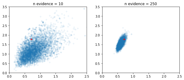
Bộ lấy mẫu HMC và NUTS thích ứng có cửa sổ

fig, ax = plt.subplots(1, 2, figsize=(10, 4))
for i, n_evidence in enumerate((10, 250)):
  ax[i].set_title(f'n evidence = {n_evidence}')
  ax[i].set_xlim(0, 2.5); ax[i].set_ylim(0, 3.5)
  @tfd.JointDistributionCoroutine
  def model():
    Root = tfd.JointDistributionCoroutine.Root
    c0 = yield Root(tfd.Gamma(2, 2, name='c0'))
    c1 = yield Root(tfd.Gamma(2, 2, name='c1'))
    counts = yield tfd.Sample(tfd.BetaBinomial(23, c1, c0), n_evidence, name='counts')
  s = model.sample(seed=[20, 30])
  print(s)
  jd = model.experimental_pin(counts=s.counts)
  states, trace = tf.function(tfp.experimental.mcmc.windowed_adaptive_hmc)(
      100, jd, num_leapfrog_steps=5, seed=[100, 200])
  ax[i].scatter(states.c0.numpy().reshape(-1), states.c1.numpy().reshape(-1), 
                marker='+', alpha=.1)
  ax[i].scatter(s.c0, s.c1, marker='+', color='r')

StructTuple(
  c0=<tf.Tensor: shape=(), dtype=float32, numpy=0.7161876>,
  c1=<tf.Tensor: shape=(), dtype=float32, numpy=1.7696666>,
  counts=<tf.Tensor: shape=(10,), dtype=float32, numpy=array([ 6., 10., 23.,  7.,  2., 20., 14., 16., 22., 17.], dtype=float32)>
)
WARNING:tensorflow:6 out of the last 6 calls to <function windowed_adaptive_hmc at 0x7fda42bed8c0> triggered tf.function retracing. Tracing is expensive and the excessive number of tracings could be due to (1) creating @tf.function repeatedly in a loop, (2) passing tensors with different shapes, (3) passing Python objects instead of tensors. For (1), please define your @tf.function outside of the loop. For (2), @tf.function has experimental_relax_shapes=True option that relaxes argument shapes that can avoid unnecessary retracing. For (3), please refer to https://www.tensorflow.org/guide/function#controlling_retracing and https://www.tensorflow.org/api_docs/python/tf/function for  more details.
StructTuple(
  c0=<tf.Tensor: shape=(), dtype=float32, numpy=0.7161876>,
  c1=<tf.Tensor: shape=(), dtype=float32, numpy=1.7696666>,
  counts=<tf.Tensor: shape=(250,), dtype=float32, numpy=
    array([ 6., 10., 23.,  7.,  2., 20., 14., 16., 22., 17., 22., 21.,  6.,
           21., 12., 22., 23., 16., 18., 21., 16., 17., 17., 16., 21., 14.,
           23., 15., 10., 19.,  8., 23., 23., 14.,  1., 23., 16., 22., 20.,
           20., 22., 15., 16., 20., 20., 21., 23., 22., 21., 15., 18., 23.,
           12., 16., 19., 23., 18.,  5., 22., 22., 22., 18., 12., 17., 17.,
           16.,  8., 22., 20., 23.,  3., 12., 14., 18.,  7., 19., 19.,  9.,
           10., 23., 14., 22., 22., 21., 13., 23., 14., 23., 10., 17., 23.,
           17., 20., 16., 20., 19., 14.,  0., 17., 22., 12.,  2., 17., 15.,
           14., 23., 19., 15., 23.,  2., 21., 23., 21.,  7., 21., 12., 23.,
           17., 17.,  4., 22., 16., 14., 19., 19., 20.,  6., 16., 14., 18.,
           21., 12., 21., 21., 22.,  2., 19., 11.,  6., 19.,  1., 23., 23.,
           14.,  6., 23., 18.,  8., 20., 23., 13., 20., 18., 23., 17., 22.,
           23., 20., 18., 22., 16., 23.,  9., 22., 21., 16., 20., 21., 16.,
           23.,  7., 13., 23., 19.,  3., 13., 23., 23., 13., 19., 23., 20.,
           18.,  8., 19., 14., 12.,  6.,  8., 23.,  3., 13., 21., 23., 22.,
           23., 19., 22., 21., 15., 22., 21., 21., 23.,  9., 19., 20., 23.,
           11., 23., 14., 23., 14., 21., 21., 10., 23.,  9., 13.,  1.,  8.,
            8., 20., 21., 21., 21., 14., 16., 16.,  9., 23., 22., 11., 23.,
           12., 18.,  1., 23.,  9.,  3., 21., 21., 23., 22., 18., 23., 16.,
            3., 11., 16.], dtype=float32)>
)

png

Toán học, số liệu thống kê

Math / linalg
- Thêm tfp.math.trapz lồng ghép hình thang.
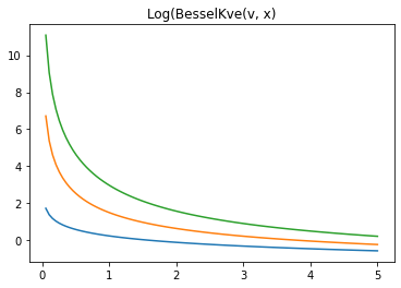
- Thêm tfp.math.log_bessel_kve .
- Thêm no_pivot_ldl để experimental.linalg .
- Thêm marginal_fn lập luận để GaussianProcess (xem no_pivot_ldl ).
- Thêm tfp.math.atan_difference(x, y)
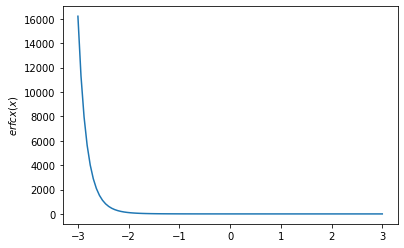
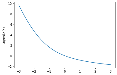
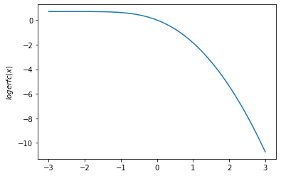
- Thêm tfp.math.erfcx , tfp.math.logerfc và tfp.math.logerfcx
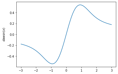
- Thêm tfp.math.dawsn cho Integral Dawson của.
- Thêm tfp.math.igammaincinv , tfp.math.igammacinv .
- Thêm tfp.math.sqrt1pm1 .
- Thêm LogitNormal.stddev_approx và LogitNormal.variance_approx
- Thêm tfp.math.owens_t cho chức năng T của Owen.
- Thêm bracket_root phương pháp để giới hạn tự động khởi tạo cho một tìm kiếm gốc.
- Thêm phương pháp của Chandrupatla để tìm gốc của các hàm vô hướng.
Số liệu thống kê
- tfp.stats.windowed_mean phương tiện hiệu quả tính cửa sổ.
- tfp.stats.windowed_variance một cách hiệu quả và chính xác tính cửa sổ chênh lệch.
- tfp.stats.cumulative_variance một cách hiệu quả và tính chính xác chênh lệch tích lũy.
- RunningCovariance và bạn bè bây giờ có thể được khởi tạo từ một ví dụ tensor, không chỉ từ hình dạng rõ ràng và dtype.
- Cleaner API cho RunningCentralMoments , RunningMean , RunningPotentialScaleReduction .

Các hàm Owen's T, Erfcx, Logerfc, Logerfcx, Dawson

# Owen's T gives the probability that X > h, 0 < Y < a * X. Let's check that
# with random sampling.
h = np.array([1., 2.]).astype(np.float32)
a = np.array([10., 11.5]).astype(np.float32)
probs = tfp.math.owens_t(h, a)

x = tfd.Normal(0., 1.).sample(int(1e5), seed=(6, 245)).numpy()
y = tfd.Normal(0., 1.).sample(int(1e5), seed=(7, 245)).numpy()

true_values = (
    (x[..., np.newaxis] > h) &
    (0. < y[..., np.newaxis]) &
    (y[..., np.newaxis] < a * x[..., np.newaxis]))

print('Calculated values: {}'.format(
    np.count_nonzero(true_values, axis=0) / 1e5))

print('Expected values: {}'.format(probs))

Calculated values: [0.07896 0.01134]
Expected values: [0.07932763 0.01137507]

x = np.linspace(-3., 3., 100)
plt.plot(x, tfp.math.erfcx(x))
plt.ylabel('$erfcx(x)$')
plt.show()

plt.plot(x, tfp.math.logerfcx(x))
plt.ylabel('$logerfcx(x)$')
plt.show()

plt.plot(x, tfp.math.logerfc(x))
plt.ylabel('$logerfc(x)$')
plt.show()

plt.plot(x, tfp.math.dawsn(x))
plt.ylabel('$dawsn(x)$')
plt.show()

png

igammainv / igammacinv

# Igammainv and Igammacinv are inverses to Igamma and Igammac

x = np.linspace(1., 10., 10)
y = tf.math.igamma(0.3, x)
x_prime = tfp.math.igammainv(0.3, y)
print('x: {}'.format(x))
print('igammainv(igamma(a, x)):\n {}'.format(x_prime))

y = tf.math.igammac(0.3, x)
x_prime = tfp.math.igammacinv(0.3, y)

print('\n')
print('x: {}'.format(x))
print('igammacinv(igammac(a, x)):\n {}'.format(x_prime))

x: [ 1.  2.  3.  4.  5.  6.  7.  8.  9. 10.]
igammainv(igamma(a, x)):
 [1.        1.9999992 3.000003  4.0000024 5.0000257 5.999887  7.0002484
 7.999243  8.99872   9.994673 ]


x: [ 1.  2.  3.  4.  5.  6.  7.  8.  9. 10.]
igammacinv(igammac(a, x)):
 [1.       2.       3.       4.       5.       6.       7.       8.000001

 9.       9.999999]

log-kve

x = np.linspace(0., 5., 100)
for v in [0.5, 2., 3]:
  plt.plot(x, tfp.math.log_bessel_kve(v, x).numpy())

plt.title('Log(BesselKve(v, x)')

Text(0.5, 1.0, 'Log(BesselKve(v, x)')

png

Khác

STS
- Đẩy nhanh tiến độ STS dự báo và phân hủy sử dụng nội tf.function gói.
- Thêm tùy chọn để tăng tốc độ lọc trong LinearGaussianSSM khi kết quả chỉ là bước cuối cùng của là bắt buộc.
- Variational Suy luận với các bản phân phối chung: ví dụ máy tính xách tay với mô hình Radon .
- Thêm hỗ trợ thử nghiệm để chuyển đổi bất kỳ phân phối nào thành một bijector điều hòa trước.
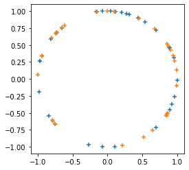
Thêm tfp.random.sanitize_seed .
Thêm tfp.random.spherical_uniform .

plt.figure(figsize=(4, 4))
seed = tfp.random.sanitize_seed(123)
seed1, seed2 = tfp.random.split_seed(seed)
samps = tfp.random.spherical_uniform([30], dimension=2, seed=seed1)
plt.scatter(*samps.numpy().T, marker='+')
samps = tfp.random.spherical_uniform([30], dimension=2, seed=seed2)
plt.scatter(*samps.numpy().T, marker='+');

png

Sổ ghi chú phát hành TFP (0.13.0)

Cài đặt và nhập

Phân phối [toán học cốt lõi]

BetaQuotient

DeterminantalPointProcess

SigmoidBeta

Zipf

NormalInverseGaussian

MatrixNormalLinearOperator

MatrixStudentTLinearOperator

Phân phối [phần mềm / wrappers]

Sharded

BatchBroadcast

Masked

Bijector

Tái cấu trúc các máy phát sinh

Sharded

VI

VI / MAP / MLE

MCMC

init_near_unconstrained_zero , retry_init

Bộ lấy mẫu HMC và NUTS thích ứng có cửa sổ

Toán học, số liệu thống kê

Các hàm Owen's T, Erfcx, Logerfc, Logerfcx, Dawson

igammainv / igammacinv

log-kve

Khác

`BetaQuotient`

`DeterminantalPointProcess`

`SigmoidBeta`

`NormalInverseGaussian`

`MatrixNormalLinearOperator`

`MatrixStudentTLinearOperator`

`Sharded`

`BatchBroadcast`

`Masked`

`Sharded`

`init_near_unconstrained_zero` , `retry_init`