TensorFlow.org에서 보기

Google Colab에서 실행

GitHub에서 소스 보기

노트북 다운로드

TensorFlow Probability를 배우기 위한 사례 연구로 이 노트북을 작성했습니다. 내가 해결하기로 선택한 문제는 2차원 평균 0 가우스 확률 변수의 샘플에 대한 공분산 행렬을 추정하는 것입니다. 이 문제에는 몇 가지 멋진 기능이 있습니다.

• 공분산에 대해 역 위시아트 사전을 사용하면(일반적인 접근 방식) 문제에 분석적 솔루션이 있으므로 결과를 확인할 수 있습니다.
• 문제는 제한된 매개변수를 샘플링하는 것과 관련되어 있어 흥미로운 복잡성을 추가합니다.
• 가장 간단한 솔루션은 가장 빠른 솔루션이 아니므로 몇 가지 최적화 작업을 수행해야 합니다.

나는 내가 따라가면서 나의 경험을 쓰기로 결정했다. TFP의 세부 사항에 대해 머리를 싸는 데 시간이 걸렸습니다. 그래서 이 노트북은 상당히 간단하게 시작하여 점차 더 복잡한 TFP 기능까지 작동합니다. 그 과정에서 많은 문제에 부딪쳤고, 문제를 식별하는 데 도움이 된 프로세스와 결국 찾은 해결 방법을 모두 캡처하려고 했습니다. 나는 (반드시 개별 단계가 올바른지 확인하기 위해 테스트를 많이 포함)의 세부 사항을 많이 포함하도록 시도했습니다.

TensorFlow 확률을 배우는 이유는 무엇입니까?

TensorFlow Probability가 다음과 같은 몇 가지 이유로 내 프로젝트에 매력적이라는 것을 알았습니다.

• TensorFlow 확률을 사용하면 노트북에서 대화형으로 복잡한 모델을 개발할 수 있는 프로토타입을 만들 수 있습니다. 코드를 단위 테스트와 대화식으로 테스트할 수 있는 작은 조각으로 나눌 수 있습니다.
• 확장할 준비가 되면 TensorFlow가 여러 컴퓨터의 최적화된 여러 프로세서에서 실행되도록 하기 위해 준비된 모든 인프라를 활용할 수 있습니다.
• 마지막으로 Stan을 정말 좋아하지만 디버깅하기가 상당히 어렵다는 것을 알게 되었습니다. 코드를 찔러보고 중간 상태를 검사하는 등의 작업을 수행할 수 있는 도구가 거의 없는 독립 실행형 언어로 모든 모델링 코드를 작성해야 합니다.

단점은 TensorFlow Probability가 Stan 및 PyMC3보다 훨씬 최신 버전이므로 문서 작업이 진행 중이고 아직 구축되지 않은 기능이 많다는 것입니다. 다행스럽게도 TFP의 기반이 탄탄하다는 것을 알게 되었고 기능을 상당히 간단하게 확장할 수 있는 모듈식 방식으로 설계되었습니다. 이 노트북에서는 사례 연구를 해결하는 것 외에도 TFP를 확장하는 몇 가지 방법을 보여 드리겠습니다.

이것은 누구를 위한 것인가

나는 독자들이 몇 가지 중요한 전제 조건을 가지고 이 노트북에 올 것이라고 가정합니다. 다음을 수행해야 합니다.

• 베이지안 추론의 기본 사항을 알고 있습니다. (그렇지 않으면, 정말 좋은 첫 번째 책은 통계 다시 생각하기 )
• MCMC 샘플링 라이브러리, 예를 들어, 어느 정도 알고 있나요 스탠 / PyMC3 / 버그
• 의 단단한 이해 되세요 NumPy와을 (하나 개의 좋은 소개입니다 파이썬은 데이터 분석을위한 )
• 와 적어도 통과 친숙에서이 TensorFlow , 그러나 반드시 전문. ( 학습 TensorFlow은 좋지만, TensorFlow의 빠른 진화 수단은 대부분의 책은 약간 일자됩니다. 스탠포드 CS20의 과정도 좋다.)

첫번째 시도

여기 문제에 대한 나의 첫 번째 시도가 있습니다. 스포일러: 내 솔루션이 작동하지 않으며 문제를 해결하려면 여러 번 시도해야 합니다! 프로세스는 시간이 걸리지만 아래의 각 시도는 TFP의 새로운 부분을 배우는 데 유용했습니다.

한 가지 참고 사항: TFP는 현재 역 Wishart 분포를 구현하지 않으므로(마지막에서 자체 역 Wishart를 실행하는 방법을 볼 것입니다) 대신 Wishart 사전을 사용하여 정밀도 행렬을 추정하는 문제로 문제를 변경할 것입니다.

import collections
import math
import os
import time

import numpy as np
import pandas as pd
import scipy
import scipy.stats
import matplotlib.pyplot as plt

import tensorflow.compat.v2 as tf
tf.enable_v2_behavior()
import tensorflow_probability as tfp
tfd = tfp.distributions
tfb = tfp.bijectors

1단계: 관찰 결과 수집

여기에 있는 내 데이터는 모두 합성 데이터이므로 실제 예제보다 약간 깔끔해 보일 것입니다. 그러나 자체 합성 데이터를 생성하지 못할 이유가 없습니다.

팁 : 모델의 형태로 결정하면, 당신은 몇 가지 매개 변수 값을 선택하고 일부 합성 데이터를 생성하기 위해 선택한 모델을 사용할 수 있습니다. 구현에 대한 온전한 검사로 선택한 매개변수의 실제 값이 추정에 포함되어 있는지 확인할 수 있습니다. 디버깅/테스트 주기를 더 빠르게 하기 위해 모델의 단순화된 버전을 고려할 수 있습니다(예: 더 적은 차원 또는 더 적은 수의 샘플 사용).

팁 : 그것은 NumPy와 배열 같은 관측 작업에 가장 쉬운 방법. 한 가지 중요한 점은 NumPy는 기본적으로 float64를 사용하는 반면 TensorFlow는 기본적으로 float32를 사용한다는 것입니다.

일반적으로 TensorFlow 작업은 모든 인수가 동일한 유형을 갖기를 원하며 유형을 변경하려면 명시적 데이터 캐스팅을 수행해야 합니다. float64 관찰을 사용하는 경우 많은 캐스트 작업을 추가해야 합니다. 대조적으로 NumPy는 자동으로 캐스팅을 처리합니다. 따라서, 사용 float64에 TensorFlow을 강제하는 것보다 float32로 NumPy와 데이터를 변환하는 것이 훨씬 쉽다.

일부 매개변수 값 선택

# We're assuming 2-D data with a known true mean of (0, 0)
true_mean = np.zeros([2], dtype=np.float32)
# We'll make the 2 coordinates correlated
true_cor = np.array([[1.0, 0.9], [0.9, 1.0]], dtype=np.float32)
# And we'll give the 2 coordinates different variances
true_var = np.array([4.0, 1.0], dtype=np.float32)
# Combine the variances and correlations into a covariance matrix
true_cov = np.expand_dims(np.sqrt(true_var), axis=1).dot(
    np.expand_dims(np.sqrt(true_var), axis=1).T) * true_cor
# We'll be working with precision matrices, so we'll go ahead and compute the
# true precision matrix here
true_precision = np.linalg.inv(true_cov)

# Here's our resulting covariance matrix
print(true_cov)
# Verify that it's positive definite, since np.random.multivariate_normal
# complains about it not being positive definite for some reason.
# (Note that I'll be including a lot of sanity checking code in this notebook -
# it's a *huge* help for debugging)
print('eigenvalues: ', np.linalg.eigvals(true_cov))

[[4.  1.8]
 [1.8 1. ]]
eigenvalues:  [4.843075   0.15692513]

일부 합성 관찰 생성

참고 TensorFlow 확률은 데이터의 초기 치수 (들) 샘플 인덱스를 대표하는 규칙을 사용하고, 데이터의 최종 치수 (들) 귀하의 샘플의 차원을 나타냅니다.

여기에서 우리는 길이의 벡터이다 각각 100 개 샘플, 2. 우리는 배열 생성 할 수 있습니다 원하는 my_data 모양 (100, 2)로한다. my_data[i, :] 는 IS \(i\)번째 샘플과 2 길이의 벡터이다.

(만들기 위해 기억 my_data 형 float32있다!)

# Set the seed so the results are reproducible.
np.random.seed(123)

# Now generate some observations of our random variable.
# (Note that I'm suppressing a bunch of spurious about the covariance matrix
# not being positive semidefinite via check_valid='ignore' because it really is
# positive definite!)
my_data = np.random.multivariate_normal(
    mean=true_mean, cov=true_cov, size=100,
    check_valid='ignore').astype(np.float32)

my_data.shape

(100, 2)

온전한 관찰 관찰

버그의 잠재적인 소스 중 하나는 합성 데이터를 엉망으로 만드는 것입니다! 몇 가지 간단한 검사를 해보자.

# Do a scatter plot of the observations to make sure they look like what we
# expect (higher variance on the x-axis, y values strongly correlated with x)
plt.scatter(my_data[:, 0], my_data[:, 1], alpha=0.75)
plt.show()

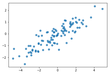
print('mean of observations:', np.mean(my_data, axis=0))
print('true mean:', true_mean)

mean of observations: [-0.24009615 -0.16638893]
true mean: [0. 0.]

print('covariance of observations:\n', np.cov(my_data, rowvar=False))
print('true covariance:\n', true_cov)

covariance of observations:
 [[3.95307734 1.68718486]
 [1.68718486 0.94910269]]
true covariance:
 [[4.  1.8]
 [1.8 1. ]]

좋아, 우리의 샘플은 합리적으로 보입니다. 다음 단계.

2단계: NumPy에서 우도 함수 구현

TF 확률에서 MCMC 샘플링을 수행하기 위해 작성해야 하는 주요 사항은 로그 가능성 함수입니다. 일반적으로 NumPy보다 TF를 작성하는 것이 약간 까다롭기 때문에 NumPy에서 초기 구현을 수행하는 것이 도움이 됩니다. I는 2 개에 대응하는 데이터의 우도 함수에 우도 함수를 분할려고 \(P(data | parameters)\) 및 사전 우도 함수는 대응하는 것을 \(P(parameters)\).

이러한 NumPy 함수는 테스트를 위해 일부 값을 생성하는 것이 목표이므로 슈퍼 최적화/벡터화할 필요가 없습니다. 정확성이 핵심 고려 사항입니다!

먼저 데이터 로그 가능성 부분을 구현합니다. 아주 간단합니다. 한 가지 기억해야 할 점은 정밀도 행렬로 작업할 것이므로 그에 따라 매개변수화할 것입니다.

def log_lik_data_numpy(precision, data):
  # np.linalg.inv is a really inefficient way to get the covariance matrix, but
  # remember we don't care about speed here
  cov = np.linalg.inv(precision)
  rv = scipy.stats.multivariate_normal(true_mean, cov)
  return np.sum(rv.logpdf(data))

# test case: compute the log likelihood of the data given the true parameters
log_lik_data_numpy(true_precision, my_data)

-280.81822950593767

우리는 후방에 대한 분석 솔루션이 이후 (참조 정밀 행렬 전에 Wishart를 사용하는거야 켤레 전과의 위키 백과의 편리한 테이블 ).

Wishart 분포는 두 매개 변수가 있습니다 :

• 자유도의 수 (표시 \(\nu\) 위키 백과)
• 스케일 매트릭스 (표지 \(V\) 위키의)

파라미터와 Wishart 분포에 대한 평균 \(\nu, V\) 있다 \(E[W] = \nu V\)및 분산은 \(\text{Var}(W_{ij}) = \nu(v_{ij}^2+v_{ii}v_{jj})\)

유용한 직관 : 당신이 발생하여 Wishart 샘플을 생성 할 수 \(\nu\) 독립적 무 \(x_1 \ldots x_{\nu}\) 0 평균 및 공분산으로 다변량 정규 확률 변수에서 \(V\) 하고 합 형성 \(W = \sum_{i=1}^{\nu} x_i x_i^T\).

당신이별로 나누어 Wishart 샘플 크기를 조정하는 경우 \(\nu\), 당신은의 샘플 공분산 행렬 얻을 \(x_i\). 이 샘플의 공분산 행렬을 향해 경향한다 \(V\) 같은 \(\nu\) 증가. 경우 \(\nu\) 작은 샘플 공분산 행렬 변동 많이 너무 작은 값있다 \(\nu\) 약한 전과 그리고 큰 값에 해당 \(\nu\) 강한 전과 대응이. 하는 것으로 \(\nu\) 적어도 당신이있는 거 샘플링 또는 단수 매트릭스를 생성 할 수 있습니다 공간의 크기와 같은 대형으로해야합니다.

우리는 사용합니다 \(\nu = 3\) 우리가 약한 이전 그래서, 우리는 할게요 \(V = \frac{1}{\nu} I\) (평균이라고 불러 신원을 향해 우리의 공분산 추정치를 끌어 \(\nu V\)).

PRIOR_DF = 3
PRIOR_SCALE = np.eye(2, dtype=np.float32) / PRIOR_DF

def log_lik_prior_numpy(precision):
  rv = scipy.stats.wishart(df=PRIOR_DF, scale=PRIOR_SCALE)
  return rv.logpdf(precision)

# test case: compute the prior for the true parameters
log_lik_prior_numpy(true_precision)

-9.103606346649766

Wishart 분포와 평균 공지 다변량 정규의 정밀도 행렬을 추정하기위한 종래 복합체이다 \(\mu\).

이전 Wishart의 매개 변수는 가정 \(\nu, V\) 우리가 가지고 \(n\) 우리의 다변량 정상, 관찰 \(x_1, \ldots, x_n\). 후방 매개 변수는 \(n + \nu, \left(V^{-1} + \sum_{i=1}^n (x_i-\mu)(x_i-\mu)^T \right)^{-1}\).

n = my_data.shape[0]
nu_prior = PRIOR_DF
v_prior = PRIOR_SCALE
nu_posterior = nu_prior + n
v_posterior = np.linalg.inv(np.linalg.inv(v_prior) + my_data.T.dot(my_data))
posterior_mean = nu_posterior * v_posterior
v_post_diag = np.expand_dims(np.diag(v_posterior), axis=1)
posterior_sd = np.sqrt(nu_posterior *
                       (v_posterior ** 2.0 + v_post_diag.dot(v_post_diag.T)))

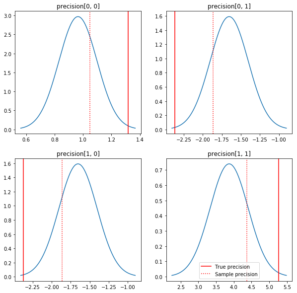
사후 및 실제 값의 빠른 플롯. 후방은 샘플 후방에 가깝지만 아이덴티티 쪽으로 약간 축소되어 있습니다. 또한 실제 값은 사후 모드와 상당히 거리가 멀다는 점에 유의하십시오. 이는 아마도 사전이 데이터와 잘 일치하지 않기 때문일 것입니다. 진짜 문제에서 우리는 가능성이 공분산을 위하여 사전 Wishart 역 스케일링 유사한 뭔가 더 할 것 (예를 들어, 참조, 앤드류 겔만의 논평 주제에),하지만 우리는 좋은 분석 후방이없는 것입니다.

sample_precision = np.linalg.inv(np.cov(my_data, rowvar=False, bias=False))
fig, axes = plt.subplots(2, 2)
fig.set_size_inches(10, 10)
for i in range(2):
  for j in range(2):
    ax = axes[i, j]
    loc = posterior_mean[i, j]
    scale = posterior_sd[i, j]
    xmin = loc - 3.0 * scale
    xmax = loc + 3.0 * scale
    x = np.linspace(xmin, xmax, 1000)
    y = scipy.stats.norm.pdf(x, loc=loc, scale=scale)
    ax.plot(x, y)
    ax.axvline(true_precision[i, j], color='red', label='True precision')
    ax.axvline(sample_precision[i, j], color='red', linestyle=':', label='Sample precision')
    ax.set_title('precision[%d, %d]' % (i, j))
plt.legend()
plt.show()

3단계: TensorFlow에서 우도 함수 구현

스포일러: 우리의 첫 번째 시도는 작동하지 않을 것입니다. 그 이유는 아래에서 이야기하겠습니다.

팁 : 사용 TensorFlow 열망 모드 당신의 가능성 기능을 개발하고 있습니다. 열망 모드는 더 NumPy와 같은 TF 동작합니다한다 - 모든 것을 실행하는 즉시, 당신이 사용하는 대신 대화 형 디버깅 할 수 있도록 Session.run() . 노트를 참조하십시오 여기를 .

예비: 배포 클래스

TFP에는 로그 확률을 생성하는 데 사용할 배포 클래스 모음이 있습니다. 한 가지 주목해야 할 점은 이러한 클래스가 단일 샘플이 아닌 샘플의 텐서와 함께 작동한다는 것입니다. 이를 통해 벡터화 및 관련 속도 향상이 가능합니다.

분포는 2가지 다른 방식으로 샘플 텐서와 함께 작동할 수 있습니다. 단일 스칼라 매개변수가 있는 분포와 관련된 구체적인 예를 통해 이 두 가지 방법을 설명하는 것이 가장 간단합니다. 내가 사용합니다 포아송 이 분포 rate 매개 변수를.

• 우리가에 대한 단일 값과 포아송를 만드는 경우 rate 매개 변수, 그에게 전화 sample() 메소드는 하나의 값을 반환합니다. 이 값은 호출 event ,이 경우 이벤트는 모든 스칼라입니다.
• 우리는 값의 텐서와 푸 아송을 만드는 경우 rate 매개 변수, 그에게 전화 sample() 메소드는 현재 속도 텐서의 각 값에 대해 하나를 여러 값을 반환합니다. 목적은 독립 물고기 자리의 컬렉션 자체 레이트 각각 역할을하고 각각의 값이 호출에 의해 리턴 된 sample() 이 물고기 자리 중 하나에 대응한다. 독립하지만 동일하게 분산 된 이벤트의이 컬렉션은라고 batch .
• sample() 메소드는 소요 sample_shape 빈 튜플에있는 기본 설정 매개 변수를. 대한 비어 있지 않은 값 전달 sample_shape 여러 배치를 돌려 샘플의 결과를. 배치의이 컬렉션은이라고 sample .

분 j의 log_prob() 메소드는 방법 평행하는 방식으로 데이터를 소모 sample() 을 생성한다. log_prob() 여러에 대한 샘플 확률, 즉, 사건의 독립적 인 배치를 돌려줍니다.

• 우리는 스칼라로 만들어진 우리의 포아송 객체가있는 경우 rate , 각 배치는 스칼라, 우리는 샘플의 텐서에 전달하면, 우리는 로그 확률의 같은 크기의 텐서을 얻을 것이다.
• 우리는 모양의 텐서로 만들어진 우리의 포아송 객체가있는 경우 T 의 rate 값을 각각 배치 모양의 텐서 T . D, T 형태의 샘플 텐서를 전달하면 D, T 형태의 로그 확률 텐서를 얻을 수 있습니다.

다음은 이러한 경우를 보여주는 몇 가지 예입니다. 참조 이 노트북을 이벤트, 배치 및 모양에 대한 더 자세한 튜토리얼.

# case 1: get log probabilities for a vector of iid draws from a single
# normal distribution
norm1 = tfd.Normal(loc=0., scale=1.)
probs1 = norm1.log_prob(tf.constant([1., 0.5, 0.]))

# case 2: get log probabilities for a vector of independent draws from
# multiple normal distributions with different parameters.  Note the vector
# values for loc and scale in the Normal constructor.
norm2 = tfd.Normal(loc=[0., 2., 4.], scale=[1., 1., 1.])
probs2 = norm2.log_prob(tf.constant([1., 0.5, 0.]))

print('iid draws from a single normal:', probs1.numpy())
print('draws from a batch of normals:', probs2.numpy())

iid draws from a single normal: [-1.4189385 -1.0439385 -0.9189385]
draws from a batch of normals: [-1.4189385 -2.0439386 -8.918939 ]

데이터 로그 가능성

먼저 데이터 로그 가능도 함수를 구현합니다.

VALIDATE_ARGS = True
ALLOW_NAN_STATS = False

NumPy 사례와의 한 가지 주요 차이점은 TensorFlow 가능도 함수가 단일 행렬이 아닌 정밀도 행렬의 벡터를 처리해야 한다는 것입니다. 여러 체인에서 샘플링할 때 매개변수 벡터가 사용됩니다.

우리는 일련의 정밀 행렬(즉, 체인당 하나의 행렬)과 함께 작동하는 분포 객체를 만들 것입니다.

데이터의 로그 확률을 계산할 때 배치 변수당 하나의 사본이 있도록 매개변수와 동일한 방식으로 데이터를 복제해야 합니다. 복제된 데이터의 모양은 다음과 같아야 합니다.

[sample shape, batch shape, event shape]

우리의 경우 이벤트 모양은 2입니다(2차원 가우시안으로 작업하기 때문에). 100개의 샘플이 있으므로 샘플 모양은 100입니다. 배치 형태는 우리가 작업하고 있는 정밀 행렬의 수일 뿐입니다. 가능성 함수를 호출할 때마다 데이터를 복제하는 것은 낭비이므로 미리 데이터를 복제하고 복제된 버전을 전달합니다.

참고이 비효율적 인 구현이다 : MultivariateNormalFullCovariance 우리가 마지막에 최적화 부분에 대해 얘기하자 몇 가지 대안에 대한 비용이 상대적입니다.

def log_lik_data(precisions, replicated_data):
  n = tf.shape(precisions)[0]  # number of precision matrices
  # We're estimating a precision matrix; we have to invert to get log
  # probabilities.  Cholesky inversion should be relatively efficient,
  # but as we'll see later, it's even better if we can avoid doing the Cholesky
  # decomposition altogether.
  precisions_cholesky = tf.linalg.cholesky(precisions)
  covariances = tf.linalg.cholesky_solve(
      precisions_cholesky, tf.linalg.eye(2, batch_shape=[n]))
  rv_data = tfd.MultivariateNormalFullCovariance(
      loc=tf.zeros([n, 2]),
      covariance_matrix=covariances,
      validate_args=VALIDATE_ARGS,
      allow_nan_stats=ALLOW_NAN_STATS)

  return tf.reduce_sum(rv_data.log_prob(replicated_data), axis=0)

# For our test, we'll use a tensor of 2 precision matrices.
# We'll need to replicate our data for the likelihood function.
# Remember, TFP wants the data to be structured so that the sample dimensions
# are first (100 here), then the batch dimensions (2 here because we have 2
# precision matrices), then the event dimensions (2 because we have 2-D
# Gaussian data).  We'll need to add a middle dimension for the batch using
# expand_dims, and then we'll need to create 2 replicates in this new dimension
# using tile.
n = 2
replicated_data = np.tile(np.expand_dims(my_data, axis=1), reps=[1, 2, 1])
print(replicated_data.shape)

(100, 2, 2)

팁 : 한 가지가 나는 내 TensorFlow 기능의 거의 정신 검사를 쓰고 매우 도움이 될 것으로 나타났습니다. TF에서 벡터화를 엉망으로 만드는 것은 정말 쉽기 때문에 더 간단한 NumPy 함수를 사용하는 것이 TF 출력을 확인하는 좋은 방법입니다. 이것을 작은 단위 테스트로 생각하십시오.

# check against the numpy implementation
precisions = np.stack([np.eye(2, dtype=np.float32), true_precision])
n = precisions.shape[0]
lik_tf = log_lik_data(precisions, replicated_data=replicated_data).numpy()

for i in range(n):
  print(i)
  print('numpy:', log_lik_data_numpy(precisions[i], my_data))
  print('tensorflow:', lik_tf[i])

0
numpy: -430.71218815801365
tensorflow: -430.71207
1
numpy: -280.81822950593767
tensorflow: -280.8182

이전 로그 가능성

데이터 복제에 대해 걱정할 필요가 없기 때문에 이전이 더 쉽습니다.

@tf.function(autograph=False)
def log_lik_prior(precisions):
  rv_precision = tfd.WishartTriL(
      df=PRIOR_DF,
      scale_tril=tf.linalg.cholesky(PRIOR_SCALE),
      validate_args=VALIDATE_ARGS,
      allow_nan_stats=ALLOW_NAN_STATS)
  return rv_precision.log_prob(precisions)

# check against the numpy implementation
precisions = np.stack([np.eye(2, dtype=np.float32), true_precision])
n = precisions.shape[0]
lik_tf = log_lik_prior(precisions).numpy()

for i in range(n):
  print(i)
  print('numpy:', log_lik_prior_numpy(precisions[i]))
  print('tensorflow:', lik_tf[i])

0
numpy: -2.2351873809649625
tensorflow: -2.2351875
1
numpy: -9.103606346649766
tensorflow: -9.103608

합동 로그 가능도 함수 작성

위의 데이터 로그 가능도 함수는 우리의 관찰에 의존하지만 샘플러에는 그런 것이 없습니다. [클로저](https://en.wikipedia.org/wiki/Closure_(computer_programming)를 사용하여 전역 변수를 사용하지 않고 종속성을 제거할 수 있습니다. 클로저는 필요한 변수를 포함하는 환경을 구축하는 외부 함수를 포함합니다. 내부 기능.

def get_log_lik(data, n_chains=1):
  # The data argument that is passed in will be available to the inner function
  # below so it doesn't have to be passed in as a parameter.
  replicated_data = np.tile(np.expand_dims(data, axis=1), reps=[1, n_chains, 1])

  @tf.function(autograph=False)
  def _log_lik(precision):
    return log_lik_data(precision, replicated_data) + log_lik_prior(precision)

  return _log_lik

4단계: 샘플

좋아, 샘플링할 시간이야! 일을 단순하게 유지하기 위해 1개의 체인만 사용하고 단위 행렬을 시작점으로 사용합니다. 우리는 나중에 더 신중하게 일을 할 것입니다.

다시 말하지만 이것은 작동하지 않을 것입니다. 예외가 발생합니다.

@tf.function(autograph=False)
def sample():
  tf.random.set_seed(123)
  init_precision = tf.expand_dims(tf.eye(2), axis=0)

  # Use expand_dims because we want to pass in a tensor of starting values
  log_lik_fn = get_log_lik(my_data, n_chains=1)

  # we'll just do a few steps here
  num_results = 10
  num_burnin_steps = 10
  states = tfp.mcmc.sample_chain(
     num_results=num_results,
     num_burnin_steps=num_burnin_steps,
     current_state=[
         init_precision,
     ],
     kernel=tfp.mcmc.HamiltonianMonteCarlo(
         target_log_prob_fn=log_lik_fn,
         step_size=0.1,
         num_leapfrog_steps=3),
     trace_fn=None,
     seed=123)
  return states

try:
  states = sample()
except Exception as e:
  # shorten the giant stack trace
  lines = str(e).split('\n')
  print('\n'.join(lines[:5]+['...']+lines[-3:]))

Cholesky decomposition was not successful. The input might not be valid.
     [[{ {node mcmc_sample_chain/trace_scan/while/body/_79/smart_for_loop/while/body/_371/mh_one_step/hmc_kernel_one_step/leapfrog_integrate/while/body/_537/leapfrog_integrate_one_step/maybe_call_fn_and_grads/value_and_gradients/StatefulPartitionedCall/Cholesky} }]] [Op:__inference_sample_2849]

Function call stack:
sample
...
Function call stack:
sample

문제 식별

InvalidArgumentError (see above for traceback): Cholesky decomposition was not successful. The input might not be valid. 별로 도움이 되지 않습니다. 무슨 일이 있었는지 자세히 알아볼까요?

• 각 단계에 대한 매개변수를 인쇄하여 실패에 대한 값을 확인할 수 있습니다.
• 특정 문제를 방지하기 위해 몇 가지 주장을 추가할 것입니다.

주장은 TensorFlow 작업이기 때문에 까다롭습니다. 그리고 우리는 그들이 실행되고 그래프에서 최적화되지 않도록 주의해야 합니다. 읽는이의 가치가 이 개요 는 TF의 주장에 익숙하지 않은 경우 TensorFlow 디버깅을. 명시 적으로 사용하여 실행하는 주장을 강제 할 수 tf.control_dependencies (아래 코드의 주석을 참조).

TensorFlow의 기본 Print 는 작업, 그리고 당신은 그것을 실행하는 것을 보장하기 위해 몇 가지주의를 취할 필요 - 기능 주장과 동일하게 작동합니다. Print 출력이 전송됩니다 : 우리가 노트북에서 작업 할 때 추가 두통의 원인 stderr 및 stderr 셀에 표시되지 않습니다. 우리는 여기에 트릭을 사용합니다 : 사용하는 대신 tf.Print , 우리를 통해 우리 자신의 TensorFlow 인쇄 작업을 만듭니다 tf.pyfunc . 주장과 마찬가지로 메서드가 실행되는지 확인해야 합니다.

def get_log_lik_verbose(data, n_chains=1):
  # The data argument that is passed in will be available to the inner function
  # below so it doesn't have to be passed in as a parameter.
  replicated_data = np.tile(np.expand_dims(data, axis=1), reps=[1, n_chains, 1])

  def _log_lik(precisions):
    # An internal method we'll make into a TensorFlow operation via tf.py_func
    def _print_precisions(precisions):
      print('precisions:\n', precisions)
      return False  # operations must return something!
    # Turn our method into a TensorFlow operation
    print_op = tf.compat.v1.py_func(_print_precisions, [precisions], tf.bool)

    # Assertions are also operations, and some care needs to be taken to ensure
    # that they're executed
    assert_op = tf.assert_equal(
        precisions, tf.linalg.matrix_transpose(precisions),
        message='not symmetrical', summarize=4, name='symmetry_check')

    # The control_dependencies statement forces its arguments to be executed
    # before subsequent operations
    with tf.control_dependencies([print_op, assert_op]):
      return (log_lik_data(precisions, replicated_data) +
              log_lik_prior(precisions))

  return _log_lik

@tf.function(autograph=False)
def sample():
  tf.random.set_seed(123)
  init_precision = tf.eye(2)[tf.newaxis, ...]
  log_lik_fn = get_log_lik_verbose(my_data)
  # we'll just do a few steps here
  num_results = 10
  num_burnin_steps = 10
  states = tfp.mcmc.sample_chain(
      num_results=num_results,
      num_burnin_steps=num_burnin_steps,
      current_state=[
          init_precision,
      ],
      kernel=tfp.mcmc.HamiltonianMonteCarlo(
          target_log_prob_fn=log_lik_fn,
          step_size=0.1,
          num_leapfrog_steps=3),
      trace_fn=None,
      seed=123)

try:
  states = sample()
except Exception as e:
  # shorten the giant stack trace
  lines = str(e).split('\n')
  print('\n'.join(lines[:5]+['...']+lines[-3:]))

precisions:
 [[[1. 0.]
  [0. 1.]]]
precisions:
 [[[1. 0.]
  [0. 1.]]]
precisions:
 [[[ 0.24315196 -0.2761638 ]
  [-0.33882257  0.8622    ]]]
 assertion failed: [not symmetrical] [Condition x == y did not hold element-wise:] [x (leapfrog_integrate_one_step/add:0) = ] [[[0.243151963 -0.276163787][-0.338822573 0.8622]]] [y (leapfrog_integrate_one_step/maybe_call_fn_and_grads/value_and_gradients/matrix_transpose/transpose:0) = ] [[[0.243151963 -0.338822573][-0.276163787 0.8622]]]
     [[{ {node mcmc_sample_chain/trace_scan/while/body/_96/smart_for_loop/while/body/_381/mh_one_step/hmc_kernel_one_step/leapfrog_integrate/while/body/_503/leapfrog_integrate_one_step/maybe_call_fn_and_grads/value_and_gradients/symmetry_check_1/Assert/AssertGuard/else/_577/Assert} }]] [Op:__inference_sample_4837]

Function call stack:
sample
...
Function call stack:
sample

이것이 실패하는 이유

샘플러가 시도하는 첫 번째 새 매개변수 값은 비대칭 행렬입니다. 대칭(및 양의 정부호) 행렬에 대해서만 정의되기 때문에 Cholesky 분해가 실패합니다.

여기서 문제는 관심 매개변수가 정밀도 행렬이고 정밀도 행렬이 실수, 대칭 및 양의 정부호여야 한다는 것입니다. 샘플러는 이 제약 조건에 대해 아무 것도 알지 못하므로(그라디언트를 통한 경우 제외) 샘플러가 잘못된 값을 제안하여 특히 단계 크기가 큰 경우 예외가 발생할 가능성이 있습니다.

Hamiltonian Monte Carlo 샘플러를 사용하면 기울기가 유효하지 않은 영역에서 매개변수를 멀리 유지해야 하지만 작은 단계 크기는 느린 수렴을 의미하므로 매우 작은 단계 크기를 사용하여 문제를 해결할 수 있습니다. 그래디언트에 대해 전혀 알지 못하는 Metropolis-Hastings 샘플러를 사용하면 우리는 운명적입니다.

버전 2: 제약이 없는 매개변수로 다시 매개변수화

위의 문제에 대한 간단한 해결책이 있습니다. 새 매개변수가 더 이상 이러한 제약 조건을 갖지 않도록 모델을 다시 매개변수화할 수 있습니다. TFP는 이를 위한 유용한 도구 세트인 바이젝터를 제공합니다.

바이젝터를 사용한 재매개변수화

우리의 정밀도 행렬은 실수와 대칭이어야 합니다. 우리는 이러한 제약이 없는 대체 매개변수화를 원합니다. 시작점은 정밀도 행렬의 Cholesky 인수분해입니다. Cholesky 요인은 여전히 ​​제한되어 있습니다. 즉, 하위 삼각형이고 대각선 요소는 양수여야 합니다. 그러나 촐레스키 인수의 대각선 로그를 취하면 로그가 더 이상 양수로 제한되지 않고 하부 삼각 부분을 1차원 벡터로 평평하게 하면 더 이상 하부 삼각 제약 조건이 없습니다. . 이 경우의 결과는 제약 조건이 없는 길이 3 벡터입니다.

합니다 ( 스탠 설명서는 매개 변수에 대한 제약 조건의 여러 유형을 제거하기 위해 변환을 사용하여에 큰 장을 가지고 있습니다.)

이 재매개변수화는 데이터 로그 가능도 함수에 거의 영향을 미치지 않습니다. 변환을 반전하면 정밀도 행렬을 다시 얻을 수 있습니다. 그러나 사전에 대한 영향은 더 복잡합니다. 우리는 주어진 정밀도 행렬의 확률이 Wishart 분포에 의해 주어지도록 지정했습니다. 변환된 행렬의 확률은 얼마입니까?

우리가 단조 함수를 적용하는 경우 호출한다는 \(g\) 1 D 랜덤 변수로 \(X\), \(Y = g(X)\)대한 밀도 \(Y\) 주어진다

\[ f_Y(y) = | \frac{d}{dy}(g^{-1}(y)) | f_X(g^{-1}(y)) \]

의 파생 \(g^{-1}\) 용어는 방식을 차지하고 \(g\) 로컬 볼륨을 변경합니다. 고차원 확률 변수의 경우, 교정 인자의 자 코비안의 결정의 절대 값 \(g^{-1}\) (참조 여기 ).

역변환의 야코비 행렬을 로그 사전 가능성 함수에 추가해야 합니다. 다행히도, TFP의 Bijector 클래스는 우리를 위해이 알아서 할 수 있습니다.

Bijector 클래스는 확률 밀도 함수의 변수를 변경하는 데 사용 가역 부드러운 함수를 나타내는데 사용된다. Bijectors는 모두가 forward() 가 행하는는 변환한다는 방법 inverse() 메소드를 그 반전 그것과 forward_log_det_jacobian() 및 inverse_log_det_jacobian() 우리가 PDF를 reparaterize 때 필요한 코비안 정정 제공 방법.

총요소 생산성은 우리가를 통해 구성을 통해 결합 할 수 있습니다 유용한 bijectors의 컬렉션을 제공 Chain 매우 복잡한 변환을 형성하는 연산자. 우리의 경우 다음 3개의 바이젝터를 구성할 것입니다(체인의 작업은 오른쪽에서 왼쪽으로 수행됨).

1. 변환의 첫 번째 단계는 정밀도 행렬에 대해 Cholesky 인수분해를 수행하는 것입니다. 이를 위한 Bijector 클래스는 없습니다. 그러나, CholeskyOuterProduct bijector 2 개 콜레 요인의 제품을합니다. 우리는 사용하여 해당 작업의 역 사용할 수 있습니다 Invert 연산자를.
2. 다음 단계는 Cholesky 요인의 대각선 요소의 로그를 취하는 것입니다. 우리는을 통해이 작업을 수행 TransformDiagonal bijector과의 역 Exp bijector.
3. 마지막으로, 우리는의 역수를 사용하여 벡터에 행렬의 하 삼각 부분을 평탄화 FillTriangular bijector한다.

# Our transform has 3 stages that we chain together via composition:
precision_to_unconstrained = tfb.Chain([
    # step 3: flatten the lower triangular portion of the matrix
    tfb.Invert(tfb.FillTriangular(validate_args=VALIDATE_ARGS)),
    # step 2: take the log of the diagonals    
    tfb.TransformDiagonal(tfb.Invert(tfb.Exp(validate_args=VALIDATE_ARGS))),
    # step 1: decompose the precision matrix into its Cholesky factors
    tfb.Invert(tfb.CholeskyOuterProduct(validate_args=VALIDATE_ARGS)),
])

# sanity checks
m = tf.constant([[1., 2.], [2., 8.]])
m_fwd = precision_to_unconstrained.forward(m)
m_inv = precision_to_unconstrained.inverse(m_fwd)

# bijectors handle tensors of values, too!
m2 = tf.stack([m, tf.eye(2)])
m2_fwd = precision_to_unconstrained.forward(m2)
m2_inv = precision_to_unconstrained.inverse(m2_fwd)

print('single input:')
print('m:\n', m.numpy())
print('precision_to_unconstrained(m):\n', m_fwd.numpy())
print('inverse(precision_to_unconstrained(m)):\n', m_inv.numpy())
print()

print('tensor of inputs:')
print('m2:\n', m2.numpy())
print('precision_to_unconstrained(m2):\n', m2_fwd.numpy())
print('inverse(precision_to_unconstrained(m2)):\n', m2_inv.numpy())

single input:
m:
 [[1. 2.]
 [2. 8.]]
precision_to_unconstrained(m):
 [0.6931472 2.        0.       ]
inverse(precision_to_unconstrained(m)):
 [[1. 2.]
 [2. 8.]]

tensor of inputs:
m2:
 [[[1. 2.]
  [2. 8.]]

 [[1. 0.]
  [0. 1.]]]
precision_to_unconstrained(m2):
 [[0.6931472 2.        0.       ]
 [0.        0.        0.       ]]
inverse(precision_to_unconstrained(m2)):
 [[[1. 2.]
  [2. 8.]]

 [[1. 0.]
  [0. 1.]]]

TransformedDistribution 클래스에 필요한 코비안 보정 분포에 bijector 적용하고 제조 공정 자동화 log_prob() . 우리의 새로운 사전은 다음과 같습니다:

def log_lik_prior_transformed(transformed_precisions):
  rv_precision = tfd.TransformedDistribution(
      tfd.WishartTriL(
          df=PRIOR_DF,
          scale_tril=tf.linalg.cholesky(PRIOR_SCALE),
          validate_args=VALIDATE_ARGS,
          allow_nan_stats=ALLOW_NAN_STATS),
      bijector=precision_to_unconstrained,
      validate_args=VALIDATE_ARGS)
  return rv_precision.log_prob(transformed_precisions)

# Check against the numpy implementation.  Note that when comparing, we need
# to add in the Jacobian correction.
precisions = np.stack([np.eye(2, dtype=np.float32), true_precision])
transformed_precisions = precision_to_unconstrained.forward(precisions)
lik_tf = log_lik_prior_transformed(transformed_precisions).numpy()
corrections = precision_to_unconstrained.inverse_log_det_jacobian(
    transformed_precisions, event_ndims=1).numpy()
n = precisions.shape[0]

for i in range(n):
  print(i)
  print('numpy:', log_lik_prior_numpy(precisions[i]) + corrections[i])
  print('tensorflow:', lik_tf[i])

0
numpy: -0.8488930160357633
tensorflow: -0.84889317
1
numpy: -7.305657151741624
tensorflow: -7.305659

데이터 로그 가능성에 대한 변환을 반전하기만 하면 됩니다.

precision = precision_to_unconstrained.inverse(transformed_precision)

우리는 실제로 정밀도 행렬의 Cholesky 인수분해를 원하기 때문에 여기에서 부분 역행렬을 수행하는 것이 더 효율적입니다. 그러나 최적화는 나중을 위해 남겨두고 부분 역행렬은 독자를 위한 연습으로 남겨 둡니다.

def log_lik_data_transformed(transformed_precisions, replicated_data):
  # We recover the precision matrix by inverting our bijector.  This is
  # inefficient since we really want the Cholesky decomposition of the
  # precision matrix, and the bijector has that in hand during the inversion,
  # but we'll worry about efficiency later.
  n = tf.shape(transformed_precisions)[0]
  precisions = precision_to_unconstrained.inverse(transformed_precisions)
  precisions_cholesky = tf.linalg.cholesky(precisions)
  covariances = tf.linalg.cholesky_solve(
      precisions_cholesky, tf.linalg.eye(2, batch_shape=[n]))
  rv_data = tfd.MultivariateNormalFullCovariance(
      loc=tf.zeros([n, 2]),
      covariance_matrix=covariances,
      validate_args=VALIDATE_ARGS,
      allow_nan_stats=ALLOW_NAN_STATS)

  return tf.reduce_sum(rv_data.log_prob(replicated_data), axis=0)

# sanity check
precisions = np.stack([np.eye(2, dtype=np.float32), true_precision])
transformed_precisions = precision_to_unconstrained.forward(precisions)
lik_tf = log_lik_data_transformed(
    transformed_precisions, replicated_data).numpy()

for i in range(precisions.shape[0]):
  print(i)
  print('numpy:', log_lik_data_numpy(precisions[i], my_data))
  print('tensorflow:', lik_tf[i])

0
numpy: -430.71218815801365
tensorflow: -430.71207
1
numpy: -280.81822950593767
tensorflow: -280.8182

다시 우리는 새로운 기능을 클로저로 감쌉니다.

def get_log_lik_transformed(data, n_chains=1):
  # The data argument that is passed in will be available to the inner function
  # below so it doesn't have to be passed in as a parameter.
  replicated_data = np.tile(np.expand_dims(data, axis=1), reps=[1, n_chains, 1])

  @tf.function(autograph=False)
  def _log_lik_transformed(transformed_precisions):
    return (log_lik_data_transformed(transformed_precisions, replicated_data) +
            log_lik_prior_transformed(transformed_precisions))

  return _log_lik_transformed

# make sure everything runs
log_lik_fn = get_log_lik_transformed(my_data)
m = tf.eye(2)[tf.newaxis, ...]
lik = log_lik_fn(precision_to_unconstrained.forward(m)).numpy()
print(lik)

[-431.5611]

견본 추출

이제 잘못된 매개변수 값으로 인해 샘플러가 폭발하는 것에 대해 걱정할 필요가 없으므로 실제 샘플을 생성해 보겠습니다.

샘플러는 매개변수의 제약 없는 버전으로 작동하므로 초기 값을 제약 없는 버전으로 변환해야 합니다. 우리가 생성하는 샘플도 모두 제약이 없는 형태이므로 다시 변환해야 합니다. 바이젝터는 벡터화되어 있으므로 쉽게 수행할 수 있습니다.

# We'll choose a proper random initial value this time
np.random.seed(123)
initial_value_cholesky = np.array(
    [[0.5 + np.random.uniform(), 0.0],
     [-0.5 + np.random.uniform(), 0.5 + np.random.uniform()]],
    dtype=np.float32)
initial_value =  initial_value_cholesky.dot(
  initial_value_cholesky.T)[np.newaxis, ...]

# The sampler works with unconstrained values, so we'll transform our initial
# value
initial_value_transformed = precision_to_unconstrained.forward(
  initial_value).numpy()

# Sample!
@tf.function(autograph=False)
def sample():
  tf.random.set_seed(123)
  log_lik_fn = get_log_lik_transformed(my_data, n_chains=1)

  num_results = 1000
  num_burnin_steps = 1000

  states, is_accepted = tfp.mcmc.sample_chain(
      num_results=num_results,
      num_burnin_steps=num_burnin_steps,
      current_state=[
          initial_value_transformed,
      ],
      kernel=tfp.mcmc.HamiltonianMonteCarlo(
          target_log_prob_fn=log_lik_fn,
          step_size=0.1,
          num_leapfrog_steps=3),
      trace_fn=lambda _, pkr: pkr.is_accepted,
      seed=123)
  # transform samples back to their constrained form
  precision_samples = [precision_to_unconstrained.inverse(s) for s in states]
  return states, precision_samples, is_accepted

states, precision_samples, is_accepted = sample()

샘플러 출력의 평균을 분석적 사후 평균과 비교합시다!

print('True posterior mean:\n', posterior_mean)
print('Sample mean:\n', np.mean(np.reshape(precision_samples, [-1, 2, 2]), axis=0))

True posterior mean:
 [[ 0.9641779 -1.6534661]
 [-1.6534661  3.8683164]]
Sample mean:
 [[ 1.4315274  -0.25587553]
 [-0.25587553  0.5740424 ]]

우리는 멀리! 이유를 알아봅시다. 먼저 샘플을 살펴보겠습니다.

np.reshape(precision_samples, [-1, 2, 2])

array([[[ 1.4315385, -0.2558777],
        [-0.2558777,  0.5740494]],

       [[ 1.4315385, -0.2558777],
        [-0.2558777,  0.5740494]],

       [[ 1.4315385, -0.2558777],
        [-0.2558777,  0.5740494]],

       ...,

       [[ 1.4315385, -0.2558777],
        [-0.2558777,  0.5740494]],

       [[ 1.4315385, -0.2558777],
        [-0.2558777,  0.5740494]],

       [[ 1.4315385, -0.2558777],
        [-0.2558777,  0.5740494]]], dtype=float32)

어 오 - 모두 같은 값을 갖는 것 같습니다. 이유를 알아봅시다.

kernel_results_ 변수는 각 상태에서 샘플러에 대한 정보를 제공하는 이름 튜플이다. is_accepted 필드는 여기에 열쇠입니다.

# Look at the acceptance for the last 100 samples
print(np.squeeze(is_accepted)[-100:])
print('Fraction of samples accepted:', np.mean(np.squeeze(is_accepted)))

[False False False False False False False False False False False False
 False False False False False False False False False False False False
 False False False False False False False False False False False False
 False False False False False False False False False False False False
 False False False False False False False False False False False False
 False False False False False False False False False False False False
 False False False False False False False False False False False False
 False False False False False False False False False False False False
 False False False False]
Fraction of samples accepted: 0.0

모든 샘플이 거부되었습니다! 아마도 우리의 단계 크기가 너무 컸습니다. 나는 선택 stepsize=0.1 순전히 임의적으로.

버전 3: 적응 단계 크기로 샘플링

내가 임의로 선택한 단계 크기로 샘플링하는 데 실패했기 때문에 몇 가지 의제 항목이 있습니다.

1. 적응 단계 크기를 구현하고
2. 몇 가지 수렴 검사를 수행합니다.

몇 가지 좋은 예제 코드가 tensorflow_probability/python/mcmc/hmc.py 적응 단계 크기를 구현하기위한이. 아래에서 수정했습니다.

별도의가 있음을 참고 sess.run() 각 단계에 대한 설명. 이것은 필요한 경우 몇 가지 단계별 진단을 쉽게 추가할 수 있기 때문에 디버깅에 정말 유용합니다. 예를 들어 증분 진행 상황, 각 단계의 시간 등을 표시할 수 있습니다.

팁 : 샘플링까지 혼란 한 가지 분명히 일반적인 방법은 루프에 그래프 성장한다을하는 것입니다. (세션이 실행되기 전에 그래프를 종료하는 이유는 바로 이러한 문제를 방지하기 위함입니다.) 하지만 finalize()를 사용하지 않은 경우 코드가 크롤링 속도가 느려지는 경우 유용한 디버깅 확인은 그래프를 인쇄하는 것입니다. 를 통해 각 단계에서 크기 len(mygraph.get_operations()) - 길이가 증가하는 경우, 당신은 아마 뭔가 나쁜 일을하고 있습니다.

여기에서 3개의 독립적인 체인을 실행할 것입니다. 체인 간의 비교를 수행하면 수렴을 확인하는 데 도움이 됩니다.

# The number of chains is determined by the shape of the initial values.
# Here we'll generate 3 chains, so we'll need a tensor of 3 initial values.
N_CHAINS = 3

np.random.seed(123)

initial_values = []
for i in range(N_CHAINS):
  initial_value_cholesky = np.array(
      [[0.5 + np.random.uniform(), 0.0],
       [-0.5 + np.random.uniform(), 0.5 + np.random.uniform()]],
      dtype=np.float32)
  initial_values.append(initial_value_cholesky.dot(initial_value_cholesky.T))
initial_values = np.stack(initial_values)

initial_values_transformed = precision_to_unconstrained.forward(
  initial_values).numpy()

@tf.function(autograph=False)
def sample():
  tf.random.set_seed(123)
  log_lik_fn = get_log_lik_transformed(my_data)

  # Tuning acceptance rates:
  dtype = np.float32
  num_burnin_iter = 3000
  num_warmup_iter = int(0.8 * num_burnin_iter) 
  num_chain_iter = 2500

  # Set the target average acceptance ratio for the HMC as suggested by
  # Beskos et al. (2013):
  # https://projecteuclid.org/download/pdfview_1/euclid.bj/1383661192
  target_accept_rate = 0.651

  # Initialize the HMC sampler.
  hmc = tfp.mcmc.HamiltonianMonteCarlo(
      target_log_prob_fn=log_lik_fn,
      step_size=0.01,
      num_leapfrog_steps=3)

  # Adapt the step size using standard adaptive MCMC procedure. See Section 4.2
  # of Andrieu and Thoms (2008):
  # http://www4.ncsu.edu/~rsmith/MA797V_S12/Andrieu08_AdaptiveMCMC_Tutorial.pdf
  adapted_kernel = tfp.mcmc.SimpleStepSizeAdaptation(
      inner_kernel=hmc,
      num_adaptation_steps=num_warmup_iter,
      target_accept_prob=target_accept_rate)

  states, is_accepted = tfp.mcmc.sample_chain(
      num_results=num_chain_iter,
      num_burnin_steps=num_burnin_iter,
      current_state=initial_values_transformed,
      kernel=adapted_kernel,
      trace_fn=lambda _, pkr: pkr.inner_results.is_accepted,
      parallel_iterations=1)
  # transform samples back to their constrained form
  precision_samples = precision_to_unconstrained.inverse(states)
  return states, precision_samples, is_accepted

states, precision_samples, is_accepted = sample()

빠른 확인: 샘플링 중 합격률은 목표인 0.651에 가깝습니다.

print(np.mean(is_accepted))

0.6190666666666667

더 좋은 점은 표본 평균과 표준 편차가 분석 솔루션에서 기대하는 것과 가깝다는 것입니다.

precision_samples_reshaped = np.reshape(precision_samples, [-1, 2, 2])
print('True posterior mean:\n', posterior_mean)
print('Mean of samples:\n', np.mean(precision_samples_reshaped, axis=0))

True posterior mean:
 [[ 0.9641779 -1.6534661]
 [-1.6534661  3.8683164]]
Mean of samples:
 [[ 0.96426415 -1.6519215 ]
 [-1.6519215   3.8614824 ]]

print('True posterior standard deviation:\n', posterior_sd)
print('Standard deviation of samples:\n', np.std(precision_samples_reshaped, axis=0))

True posterior standard deviation:
 [[0.13435492 0.25050813]
 [0.25050813 0.53903675]]
Standard deviation of samples:
 [[0.13622096 0.25235635]
 [0.25235635 0.5394968 ]]

수렴 확인

일반적으로 확인할 분석 솔루션이 없으므로 샘플러가 수렴되었는지 확인해야 합니다. 하나의 표준 검사는 겔만 - 루빈입니다 \(\hat{R}\) 여러 샘플링 체인을 필요로 통계. \(\hat{R}\) 측정 정도는 체인 사이에있는 차이 (수단의)에 체인이 동일하게 분산 된 경우 하나가 무엇을 기대 초과합니다. 값 \(\hat{R}\) 1 가까이 근접한 수렴을 나타내는 데 사용된다. 참조 소스 자세한 내용을.

r_hat = tfp.mcmc.potential_scale_reduction(precision_samples).numpy()
print(r_hat)

[[1.0038308 1.0005717]
 [1.0005717 1.0006068]]

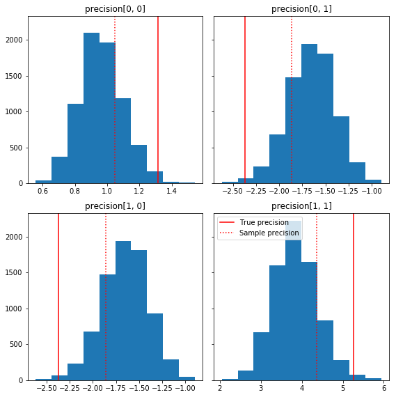
모델 비평

분석적 솔루션이 없었다면 지금이 실제 모델 비판을 할 때였을 것입니다.

다음은 실측(빨간색)과 관련된 샘플 구성 요소의 몇 가지 빠른 히스토그램입니다. 샘플은 샘플 정밀도 행렬 값에서 단위 행렬 이전으로 축소되었습니다.

fig, axes = plt.subplots(2, 2, sharey=True)
fig.set_size_inches(8, 8)
for i in range(2):
  for j in range(2):
    ax = axes[i, j]
    ax.hist(precision_samples_reshaped[:, i, j])
    ax.axvline(true_precision[i, j], color='red',
               label='True precision')
    ax.axvline(sample_precision[i, j], color='red', linestyle=':',
               label='Sample precision')
    ax.set_title('precision[%d, %d]' % (i, j))
plt.tight_layout()
plt.legend()
plt.show()

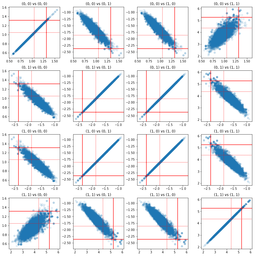
정밀도 구성요소 쌍의 일부 산점도는 사후의 상관 구조로 인해 실제 사후 값이 위의 주변부에서 나타나는 것만큼 가능성이 낮지 않다는 것을 보여줍니다.

fig, axes = plt.subplots(4, 4)
fig.set_size_inches(12, 12)
for i1 in range(2):
  for j1 in range(2):
    index1 = 2 * i1 + j1
    for i2 in range(2):
      for j2 in range(2):
        index2 = 2 * i2 + j2
        ax = axes[index1, index2]
        ax.scatter(precision_samples_reshaped[:, i1, j1],
                   precision_samples_reshaped[:, i2, j2], alpha=0.1)
        ax.axvline(true_precision[i1, j1], color='red')
        ax.axhline(true_precision[i2, j2], color='red')
        ax.axvline(sample_precision[i1, j1], color='red', linestyle=':')
        ax.axhline(sample_precision[i2, j2], color='red', linestyle=':')
        ax.set_title('(%d, %d) vs (%d, %d)' % (i1, j1, i2, j2))
plt.tight_layout()
plt.show()

버전 4: 제한된 매개변수의 더 간단한 샘플링

Bijector는 정밀 행렬 샘플링을 간단하게 만들었지만 제약이 없는 표현으로 또는 그 반대로 수동으로 변환하는 작업이 상당히 많았습니다. 더 쉬운 방법이 있습니다!

TransformedTransitionKernel

TransformedTransitionKernel 이 과정을 단순화합니다. 샘플러를 래핑하고 모든 변환을 처리합니다. 제약이 없는 매개변수 값을 제약이 있는 매개변수 값으로 매핑하는 바이젝터 목록을 인수로 취합니다. 그래서 여기에 우리는의 역이 필요 precision_to_unconstrained 위에서 사용 bijector합니다. 우리는 사용할 수 tfb.Invert(precision_to_unconstrained) ,하지만 그 역함수의 역함수를 받기 포함 것 (TensorFlow 단순화하는 스마트 것만으로는 충분하지 않습니다 tf.Invert(tf.Invert()) 에 tf.Identity()) , 그래서 대신에 우리 그냥 새로운 bijector를 쓸거야.

바이젝터 구속

# The bijector we need for the TransformedTransitionKernel is the inverse of
# the one we used above
unconstrained_to_precision = tfb.Chain([
    # step 3: take the product of Cholesky factors
    tfb.CholeskyOuterProduct(validate_args=VALIDATE_ARGS),
    # step 2: exponentiate the diagonals    
    tfb.TransformDiagonal(tfb.Exp(validate_args=VALIDATE_ARGS)),
    # step 1: map a vector to a lower triangular matrix
    tfb.FillTriangular(validate_args=VALIDATE_ARGS),
])

# quick sanity check
m = [[1., 2.], [2., 8.]]
m_inv = unconstrained_to_precision.inverse(m).numpy()
m_fwd = unconstrained_to_precision.forward(m_inv).numpy()

print('m:\n', m)
print('unconstrained_to_precision.inverse(m):\n', m_inv)
print('forward(unconstrained_to_precision.inverse(m)):\n', m_fwd)

m:
 [[1.0, 2.0], [2.0, 8.0]]
unconstrained_to_precision.inverse(m):
 [0.6931472 2.        0.       ]
forward(unconstrained_to_precision.inverse(m)):
 [[1. 2.]
 [2. 8.]]

TransformedTransitionKernel을 사용한 샘플링

으로 TransformedTransitionKernel , 우리는 더 이상 우리의 매개 변수를 수동으로 변환을 할 필요가 없습니다. 초기 값과 샘플은 모두 정밀도 행렬입니다. 우리는 제약 없는 바이젝터를 커널에 전달하기만 하면 됩니다. 그러면 커널이 모든 변환을 처리합니다.

@tf.function(autograph=False)
def sample():
  tf.random.set_seed(123)
  log_lik_fn = get_log_lik(my_data)

  # Tuning acceptance rates:
  dtype = np.float32
  num_burnin_iter = 3000
  num_warmup_iter = int(0.8 * num_burnin_iter) 
  num_chain_iter = 2500

  # Set the target average acceptance ratio for the HMC as suggested by
  # Beskos et al. (2013):
  # https://projecteuclid.org/download/pdfview_1/euclid.bj/1383661192
  target_accept_rate = 0.651

  # Initialize the HMC sampler.
  hmc = tfp.mcmc.HamiltonianMonteCarlo(
      target_log_prob_fn=log_lik_fn,
      step_size=0.01,
      num_leapfrog_steps=3)

  ttk = tfp.mcmc.TransformedTransitionKernel(
      inner_kernel=hmc, bijector=unconstrained_to_precision)

  # Adapt the step size using standard adaptive MCMC procedure. See Section 4.2
  # of Andrieu and Thoms (2008):
  # http://www4.ncsu.edu/~rsmith/MA797V_S12/Andrieu08_AdaptiveMCMC_Tutorial.pdf
  adapted_kernel = tfp.mcmc.SimpleStepSizeAdaptation(
      inner_kernel=ttk,
      num_adaptation_steps=num_warmup_iter,
      target_accept_prob=target_accept_rate)

  states = tfp.mcmc.sample_chain(
      num_results=num_chain_iter,
      num_burnin_steps=num_burnin_iter,
      current_state=initial_values,
      kernel=adapted_kernel,
      trace_fn=None,
      parallel_iterations=1)
  # transform samples back to their constrained form
  return states

precision_samples  = sample()

수렴 확인

\(\hat{R}\) 컨버전스 체크 외모 좋은!

r_hat = tfp.mcmc.potential_scale_reduction(precision_samples).numpy()
print(r_hat)

[[1.0013582 1.0019467]
 [1.0019467 1.0011805]]

사후분석과의 비교

다시 분석적 사후에 대해 확인합시다.

# The output samples have shape [n_steps, n_chains, 2, 2]
# Flatten them to [n_steps * n_chains, 2, 2] via reshape:
precision_samples_reshaped = np.reshape(precision_samples, [-1, 2, 2])

print('True posterior mean:\n', posterior_mean)
print('Mean of samples:\n', np.mean(precision_samples_reshaped, axis=0))

True posterior mean:
 [[ 0.9641779 -1.6534661]
 [-1.6534661  3.8683164]]
Mean of samples:
 [[ 0.96687526 -1.6552585 ]
 [-1.6552585   3.867676  ]]

print('True posterior standard deviation:\n', posterior_sd)
print('Standard deviation of samples:\n', np.std(precision_samples_reshaped, axis=0))

True posterior standard deviation:
 [[0.13435492 0.25050813]
 [0.25050813 0.53903675]]
Standard deviation of samples:
 [[0.13329624 0.24913791]
 [0.24913791 0.53983927]]

최적화

이제 엔드 투 엔드 실행이 완료되었으므로 더 최적화된 버전을 만들어 보겠습니다. 이 예에서는 속도가 그다지 중요하지 않지만 일단 행렬이 커지면 몇 가지 최적화가 큰 차이를 만들 것입니다.

우리가 할 수 있는 한 가지 큰 속도 개선은 Cholesky 분해의 관점에서 다시 매개변수화하는 것입니다. 그 이유는 데이터 우도 함수에 공분산과 정밀도 행렬이 모두 필요하기 때문입니다. 매트릭스 반전 비싼이다 (\(O(n^3)\) 에 대한 \(n \times n\) 매트릭스), 우리는 공분산 또는 정밀 매트릭스 중 하나의 관점에서 매개 변수화 할 경우, 우리는 서로를 얻을 수있는 반전을 할 필요가있다.

알림 등의 실제 포지티브 명확한 대칭 행렬 \(M\) 폼의 곱으로 분해 될 수 \(M = L L^T\) 매트릭스 \(L\) 하부 삼각형 긍정적 대각선을 갖는다. 의 촐레 스키 분해를 감안 \(M\), 우리는보다 효율적 모두 얻을 수 \(M\) (하부의 생성물과 상 삼각 행렬)과 \(M^{-1}\) (백 교체를 통해). 촐레스키 인수분해 자체는 계산하기에 저렴하지 않지만 촐레스키 인수로 매개변수화하면 초기 매개변수 값의 촐렉시 인수분해만 계산하면 됩니다.

공분산 행렬의 촐레스키 분해 사용

TFP는 다변량 정규 분포의 버전은 MultivariateNormalTriL 공분산 행렬의 촐레 스키 인자의 관점에서 파라미터 화된다. 따라서 공분산 행렬의 촐레스키 인수로 매개변수화하면 데이터 로그 가능성을 효율적으로 계산할 수 있습니다. 문제는 유사한 효율성으로 이전 로그 가능성을 계산하는 것입니다.

샘플의 촐레스키 인수와 함께 작동하는 역 Wishart 분포 버전이 있다면 모든 것이 설정되었을 것입니다. 아아, 우리는하지 않습니다. (하지만 팀은 코드 제출을 환영합니다!) 대안으로 바이젝터 체인과 함께 샘플의 Cholesky 인수와 함께 작동하는 Wishart 배포 버전을 사용할 수 있습니다.

현재 우리는 일을 정말 효율적으로 만들기 위해 몇 개의 스톡 바이젝터를 놓치고 있지만, 저는 TFP 바이젝터의 위력에 대한 유용한 예시이자 연습으로 프로세스를 보여주고 싶습니다.

촐레스키 요인에 대해 작동하는 Wishart 분포

Wishart 분포 유용한 플래그가 input_output_cholesky 지정 입력 및 출력 행렬을 촐레 스키 인자되어야한다는 것을. 전체 행렬보다 촐레스키 인수로 작업하는 것이 더 효율적이고 수치적으로 유리하므로 이것이 바람직한 이유입니다. 플래그의 의미에 대한 중요한 점은 : 그 분포에 대한 입력 및 출력의 표현을 변경한다고 만 표시이다 - 그것은에 코비안 보정 포함 할 분포의 전체 변수화 나타내지 않는다 log_prob() 기능. 우리는 실제로 이 전체 재매개변수화를 수행하기를 원하므로 자체 배포를 구축할 것입니다.

# An optimized Wishart distribution that has been transformed to operate on
# Cholesky factors instead of full matrices.  Note that we gain a modest
# additional speedup by specifying the Cholesky factor of the scale matrix
# (i.e. by passing in the scale_tril parameter instead of scale).

class CholeskyWishart(tfd.TransformedDistribution):
  """Wishart distribution reparameterized to use Cholesky factors."""
  def __init__(self,
      df,
      scale_tril,
      validate_args=False,
      allow_nan_stats=True,
      name='CholeskyWishart'):
    # Wishart has a bunch of methods that we want to support but not
    # implement.  We'll subclass TransformedDistribution here to take care of
    # those.  We'll override the few for which speed is critical and implement
    # them with a separate Wishart for which input_output_cholesky=True
    super(CholeskyWishart, self).__init__(
        distribution=tfd.WishartTriL(
            df=df,
            scale_tril=scale_tril,
            input_output_cholesky=False,
            validate_args=validate_args,
            allow_nan_stats=allow_nan_stats),
        bijector=tfb.Invert(tfb.CholeskyOuterProduct()),
        validate_args=validate_args,
        name=name
    )
    # Here's the Cholesky distribution we'll use for log_prob() and sample()
    self.cholesky = tfd.WishartTriL(
        df=df,
        scale_tril=scale_tril,
        input_output_cholesky=True,
        validate_args=validate_args,
        allow_nan_stats=allow_nan_stats)

  def _log_prob(self, x):
    return (self.cholesky.log_prob(x) +
            self.bijector.inverse_log_det_jacobian(x, event_ndims=2))

  def _sample_n(self, n, seed=None):
    return self.cholesky._sample_n(n, seed)

# some checks
PRIOR_SCALE_CHOLESKY = np.linalg.cholesky(PRIOR_SCALE)

@tf.function(autograph=False)
def compute_log_prob(m):
  w_transformed = tfd.TransformedDistribution(
      tfd.WishartTriL(df=PRIOR_DF, scale_tril=PRIOR_SCALE_CHOLESKY),
      bijector=tfb.Invert(tfb.CholeskyOuterProduct()))
  w_optimized = CholeskyWishart(
      df=PRIOR_DF, scale_tril=PRIOR_SCALE_CHOLESKY)
  log_prob_transformed = w_transformed.log_prob(m)
  log_prob_optimized = w_optimized.log_prob(m)
  return log_prob_transformed, log_prob_optimized

for matrix in [np.eye(2, dtype=np.float32),
               np.array([[1., 0.], [2., 8.]], dtype=np.float32)]:
  log_prob_transformed, log_prob_optimized = [
      t.numpy() for t in compute_log_prob(matrix)]
  print('Transformed Wishart:', log_prob_transformed)
  print('Optimized Wishart', log_prob_optimized)

Transformed Wishart: -0.84889317
Optimized Wishart -0.84889317
Transformed Wishart: -99.269455
Optimized Wishart -99.269455

역 Wishart 분포 구축

우리는 우리의 공분산 행렬이 \(C\) 로 분해 \(C = L L^T\) \(L\) 낮은 삼각형이고 긍정적 인 대각선이있다. 우리의 확률을 알고 싶어 \(L\) 주어진 \(C \sim W^{-1}(\nu, V)\) 곳 \(W^{-1}\) Wishart 배포 역입니다.

역 Wishart 분포 특성을 갖는다 경우 \(C \sim W^{-1}(\nu, V)\)후 정밀 매트릭스 \(C^{-1} \sim W(\nu, V^{-1})\). 그래서 우리는 확률 얻을 수 \(L\) 비아 TransformedDistribution 매개 변수로 Wishart 분포와 그 역의 콜레 요인에 정밀 행렬의 콜레 요소를 매핑하는 bijector 걸립니다.

의 콜레 인자에서 얻을 수있는 간단한 (하지만 매우 효율적이지) 방법 \(C^{-1}\) 에 \(L\) 다음이 반전 요소의 공분산 행렬을 형성 한 다음 콜레 인수 분해를하고, 다시 해결하여 콜레 계수를 반전하는 것입니다 .

의 콜레 분해하자 \(C^{-1} = M M^T\). \(M\) 우리가 사용하여 반전 할 수 있도록 낮은 삼각형 MatrixInverseTriL bijector을.

성형 \(C\) 에서 \(M^{-1}\) : 조금 까다 롭습니다 \(C = (M M^T)^{-1} = M^{-T}M^{-1} = M^{-T} (M^{-T})^T\). \(M\) 되도록, 하부 삼각형 \(M^{-1}\) 또한 하 삼각 것이며, \(M^{-T}\) 상 삼각 것이다. CholeskyOuterProduct() 우리가 형성하는 데 사용할 수 없도록 bijector 만 낮은 삼각 행렬과 함께 작동 \(C\) 에서 \(M^{-T}\). 우리의 해결 방법은 행렬의 행과 열을 치환하는 일련의 바이젝터입니다.

다행히이 논리는 캡슐화되어 CholeskyToInvCholesky bijector!

모든 조각을 결합

# verify that the bijector works
m = np.array([[1., 0.], [2., 8.]], dtype=np.float32)
c_inv = m.dot(m.T)
c = np.linalg.inv(c_inv)
c_chol = np.linalg.cholesky(c)
wishart_cholesky_to_iw_cholesky = tfb.CholeskyToInvCholesky()
w_fwd = wishart_cholesky_to_iw_cholesky.forward(m).numpy()

print('numpy =\n', c_chol)
print('bijector =\n', w_fwd)

numpy =
 [[ 1.0307764   0.        ]
 [-0.03031695  0.12126781]]
bijector =
 [[ 1.0307764   0.        ]
 [-0.03031695  0.12126781]]

우리의 최종 배포

Cholesky 요인에 대해 작동하는 역 Wishart는 다음과 같습니다.

inverse_wishart_cholesky = tfd.TransformedDistribution(
    distribution=CholeskyWishart(
        df=PRIOR_DF,
        scale_tril=np.linalg.cholesky(np.linalg.inv(PRIOR_SCALE))),
    bijector=tfb.CholeskyToInvCholesky())

역위시아트가 있지만 바이젝터에서 촐레스키 분해를 해야 하기 때문에 속도가 좀 느립니다. 정밀 행렬 매개변수화로 돌아가서 최적화를 위해 무엇을 할 수 있는지 봅시다.

Final(!) 버전: 정밀도 행렬의 Cholesky 분해 사용

다른 접근 방식은 정밀도 행렬의 촐레스키 인수로 작업하는 것입니다. 여기서 사전 가능성 함수는 계산하기 쉽지만 TFP에는 정밀도로 매개변수화된 다변량 법선 버전이 없기 때문에 데이터 로그 가능성 함수는 더 많은 작업이 필요합니다.

최적화된 사전 로그 가능성

우리는 사용 CholeskyWishart 우리가 이전을 구성하기 위해 위의 내장 분포를.

# Our new prior.
PRIOR_SCALE_CHOLESKY = np.linalg.cholesky(PRIOR_SCALE)

def log_lik_prior_cholesky(precisions_cholesky):
  rv_precision = CholeskyWishart(
      df=PRIOR_DF,
      scale_tril=PRIOR_SCALE_CHOLESKY,
      validate_args=VALIDATE_ARGS,
      allow_nan_stats=ALLOW_NAN_STATS)
  return rv_precision.log_prob(precisions_cholesky)

# Check against the slower TF implementation and the NumPy implementation.
# Note that when comparing to NumPy, we need to add in the Jacobian correction.
precisions = [np.eye(2, dtype=np.float32),
              true_precision]
precisions_cholesky = np.stack([np.linalg.cholesky(m) for m in precisions])
precisions = np.stack(precisions)
lik_tf = log_lik_prior_cholesky(precisions_cholesky).numpy()
lik_tf_slow = tfd.TransformedDistribution(
    distribution=tfd.WishartTriL(
        df=PRIOR_DF, scale_tril=tf.linalg.cholesky(PRIOR_SCALE)),
    bijector=tfb.Invert(tfb.CholeskyOuterProduct())).log_prob(
    precisions_cholesky).numpy()
corrections = tfb.Invert(tfb.CholeskyOuterProduct()).inverse_log_det_jacobian(
    precisions_cholesky, event_ndims=2).numpy()
n = precisions.shape[0]

for i in range(n):
  print(i)
  print('numpy:', log_lik_prior_numpy(precisions[i]) + corrections[i])
  print('tensorflow slow:', lik_tf_slow[i])
  print('tensorflow fast:', lik_tf[i])

0
numpy: -0.8488930160357633
tensorflow slow: -0.84889317
tensorflow fast: -0.84889317
1
numpy: -7.442875031036973
tensorflow slow: -7.442877
tensorflow fast: -7.442876

Optimized data log likelihood

We can use TFP's bijectors to build our own version of the multivariate normal. Here is the key idea:

Suppose I have a column vector \(X\) whose elements are iid samples of \(N(0, 1)\). We have \(\text{mean}(X) = 0\) and \(\text{cov}(X) = I\)

Now let \(Y = A X + b\). We have \(\text{mean}(Y) = b\) and \(\text{cov}(Y) = A A^T\)

Hence we can make vectors with mean \(b\) and covariance \(C\) using the affine transform \(Ax+b\) to vectors of iid standard Normal samples provided \(A A^T = C\). The Cholesky decomposition of \(C\) has the desired property. However, there are other solutions.

Let \(P = C^{-1}\) and let the Cholesky decomposition of \(P\) be \(B\), ie \(B B^T = P\). Now

\(P^{-1} = (B B^T)^{-1} = B^{-T} B^{-1} = B^{-T} (B^{-T})^T\)

So another way to get our desired mean and covariance is to use the affine transform \(Y=B^{-T}X + b\).

Our approach (courtesy of this notebook ):

1. Use tfd.Independent() to combine a batch of 1-D Normal random variables into a single multi-dimensional random variable. The reinterpreted_batch_ndims parameter for Independent() specifies the number of batch dimensions that should be reinterpreted as event dimensions. In our case we create a 1-D batch of length 2 that we transform into a 1-D event of length 2, so reinterpreted_batch_ndims=1 .
2. Apply a bijector to add the desired covariance: tfb.Invert(tfb.ScaleMatvecTriL(scale_tril=precision_cholesky, adjoint=True)) . Note that above we're multiplying our iid normal random variables by the transpose of the inverse of the Cholesky factor of the precision matrix \((B^{-T}X)\). The tfb.Invert takes care of inverting \(B\), and the adjoint=True flag performs the transpose.
3. Apply a bijector to add the desired offset: tfb.Shift(shift=shift) Note that we have to do the shift as a separate step from the initial inverted affine transform because otherwise the inverted scale is applied to the shift (since the inverse of \(y=Ax+b\) is \(x=A^{-1}y - A^{-1}b\)).

class MVNPrecisionCholesky(tfd.TransformedDistribution):
  """Multivariate normal parameterized by loc and Cholesky precision matrix."""

  def __init__(self, loc, precision_cholesky, name=None):
    super(MVNPrecisionCholesky, self).__init__(
        distribution=tfd.Independent(
            tfd.Normal(loc=tf.zeros_like(loc),
                       scale=tf.ones_like(loc)),
            reinterpreted_batch_ndims=1),
        bijector=tfb.Chain([
            tfb.Shift(shift=loc),
            tfb.Invert(tfb.ScaleMatvecTriL(scale_tril=precision_cholesky,
                                  adjoint=True)),
        ]),
        name=name)

@tf.function(autograph=False)
def log_lik_data_cholesky(precisions_cholesky, replicated_data):
  n = tf.shape(precisions_cholesky)[0]  # number of precision matrices
  rv_data = MVNPrecisionCholesky(
      loc=tf.zeros([n, 2]),
      precision_cholesky=precisions_cholesky)
  return tf.reduce_sum(rv_data.log_prob(replicated_data), axis=0)

# check against the numpy implementation
true_precision_cholesky = np.linalg.cholesky(true_precision)
precisions = [np.eye(2, dtype=np.float32), true_precision]
precisions_cholesky = np.stack([np.linalg.cholesky(m) for m in precisions])
precisions = np.stack(precisions)
n = precisions_cholesky.shape[0]
replicated_data = np.tile(np.expand_dims(my_data, axis=1), reps=[1, 2, 1])
lik_tf = log_lik_data_cholesky(precisions_cholesky, replicated_data).numpy()

for i in range(n):
  print(i)
  print('numpy:', log_lik_data_numpy(precisions[i], my_data))
  print('tensorflow:', lik_tf[i])

0
numpy: -430.71218815801365
tensorflow: -430.71207
1
numpy: -280.81822950593767
tensorflow: -280.81824

Combined log likelihood function

Now we combine our prior and data log likelihood functions in a closure.

def get_log_lik_cholesky(data, n_chains=1):
  # The data argument that is passed in will be available to the inner function
  # below so it doesn't have to be passed in as a parameter.
  replicated_data = np.tile(np.expand_dims(data, axis=1), reps=[1, n_chains, 1])

  @tf.function(autograph=False)
  def _log_lik_cholesky(precisions_cholesky):
    return (log_lik_data_cholesky(precisions_cholesky, replicated_data) +
            log_lik_prior_cholesky(precisions_cholesky))

  return _log_lik_cholesky

Constraining bijector

Our samples are constrained to be valid Cholesky factors, which means they must be lower triangular matrices with positive diagonals. The TransformedTransitionKernel needs a bijector that maps unconstrained tensors to/from tensors with our desired constraints. We've removed the Cholesky decomposition from the bijector's inverse, which speeds things up.

unconstrained_to_precision_cholesky = tfb.Chain([
    # step 2: exponentiate the diagonals    
    tfb.TransformDiagonal(tfb.Exp(validate_args=VALIDATE_ARGS)),
    # step 1: expand the vector to a lower triangular matrix
    tfb.FillTriangular(validate_args=VALIDATE_ARGS),
])

# some checks
inv = unconstrained_to_precision_cholesky.inverse(precisions_cholesky).numpy()
fwd = unconstrained_to_precision_cholesky.forward(inv).numpy()
print('precisions_cholesky:\n', precisions_cholesky)
print('\ninv:\n', inv)
print('\nfwd(inv):\n', fwd)

precisions_cholesky:
 [[[ 1.         0.       ]
  [ 0.         1.       ]]

 [[ 1.1470785  0.       ]
  [-2.0647411  1.0000004]]]

inv:
 [[ 0.0000000e+00  0.0000000e+00  0.0000000e+00]
 [ 3.5762781e-07 -2.0647411e+00  1.3721828e-01]]

fwd(inv):
 [[[ 1.         0.       ]
  [ 0.         1.       ]]

 [[ 1.1470785  0.       ]
  [-2.0647411  1.0000004]]]

Initial values

We generate a tensor of initial values. We're working with Cholesky factors, so we generate some Cholesky factor initial values.

# The number of chains is determined by the shape of the initial values.
# Here we'll generate 3 chains, so we'll need a tensor of 3 initial values.
N_CHAINS = 3

np.random.seed(123)

initial_values_cholesky = []
for i in range(N_CHAINS):
  initial_values_cholesky.append(np.array(
      [[0.5 + np.random.uniform(), 0.0],
       [-0.5 + np.random.uniform(), 0.5 + np.random.uniform()]],
      dtype=np.float32))
initial_values_cholesky = np.stack(initial_values_cholesky)

Sampling

We sample N_CHAINS chains using the TransformedTransitionKernel .

@tf.function(autograph=False)
def sample():
  tf.random.set_seed(123)
  log_lik_fn = get_log_lik_cholesky(my_data)

  # Tuning acceptance rates:
  dtype = np.float32
  num_burnin_iter = 3000
  num_warmup_iter = int(0.8 * num_burnin_iter) 
  num_chain_iter = 2500

  # Set the target average acceptance ratio for the HMC as suggested by
  # Beskos et al. (2013):
  # https://projecteuclid.org/download/pdfview_1/euclid.bj/1383661192
  target_accept_rate = 0.651

  # Initialize the HMC sampler.
  hmc = tfp.mcmc.HamiltonianMonteCarlo(
      target_log_prob_fn=log_lik_fn,
      step_size=0.01,
      num_leapfrog_steps=3)

  ttk = tfp.mcmc.TransformedTransitionKernel(
      inner_kernel=hmc, bijector=unconstrained_to_precision_cholesky)

  # Adapt the step size using standard adaptive MCMC procedure. See Section 4.2
  # of Andrieu and Thoms (2008):
  # http://www4.ncsu.edu/~rsmith/MA797V_S12/Andrieu08_AdaptiveMCMC_Tutorial.pdf
  adapted_kernel = tfp.mcmc.SimpleStepSizeAdaptation(
      inner_kernel=ttk,
      num_adaptation_steps=num_warmup_iter,
      target_accept_prob=target_accept_rate)

  states = tfp.mcmc.sample_chain(
      num_results=num_chain_iter,
      num_burnin_steps=num_burnin_iter,
      current_state=initial_values,
      kernel=adapted_kernel,
      trace_fn=None,
      parallel_iterations=1)
  # transform samples back to their constrained form
  samples = tf.linalg.matmul(states, states, transpose_b=True)
  return samples

precision_samples = sample()

Convergence check

A quick convergence check looks good:

r_hat = tfp.mcmc.potential_scale_reduction(precision_samples).numpy()
print(r_hat)

[[1.0013583 1.0019467]
 [1.0019467 1.0011804]]

Comparing results to the analytic posterior

# The output samples have shape [n_steps, n_chains, 2, 2]
# Flatten them to [n_steps * n_chains, 2, 2] via reshape:
precision_samples_reshaped = np.reshape(precision_samples, newshape=[-1, 2, 2])

And again, the sample means and standard deviations match those of the analytic posterior.

print('True posterior mean:\n', posterior_mean)
print('Mean of samples:\n', np.mean(precision_samples_reshaped, axis=0))

True posterior mean:
 [[ 0.9641779 -1.6534661]
 [-1.6534661  3.8683164]]
Mean of samples:
 [[ 0.9668749 -1.6552604]
 [-1.6552604  3.8676758]]

print('True posterior standard deviation:\n', posterior_sd)
print('Standard deviation of samples:\n', np.std(precision_samples_reshaped, axis=0))

True posterior standard deviation:
 [[0.13435492 0.25050813]
 [0.25050813 0.53903675]]
Standard deviation of samples:
 [[0.13329637 0.24913797]
 [0.24913797 0.53983945]]

Ok, all done! We've got our optimized sampler working.